The Deleted Degrees of Freedom: A Case for Potential-Primary Electrodynamics
Dr. Paul Wilhelm1, Advanced Rediscovery2 · 2026-03-19EM Foundations
1 Introduction
The question of whether the vector potential \(\mathbf{A}\) is physically real was settled experimentally in 1986 [1]. The question of what was lost when physics declared it auxiliary has barely been asked.
The standard formulation of classical electrodynamics treats electric and magnetic fields \(\mathbf{E}\) and \(\mathbf{B}\) as the fundamental physical quantities, with the potentials \(\phi\) and \(\mathbf{A}\) serving as computational tools. This hierarchy was not discovered. It was constructed — through two deliberate 19th-century simplifications and one philosophical decision that subsequent generations inherited without re-examination.
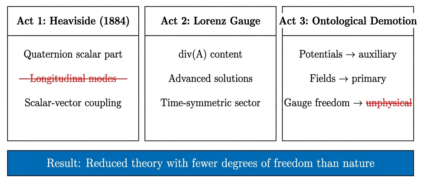
Each simplification deleted physical content. Heaviside’s vector reduction [2] eliminated the scalar part of Maxwell’s quaternion formulation, discarding longitudinal modes and the scalar-vector coupling terms. The Lorenz gauge convention suppressed the independent content of \(\nabla \cdot \mathbf{A}\) and discarded advanced solutions. The resulting ontological consensus — that fields are primary and potentials auxiliary — was a philosophical choice dressed as an empirical conclusion.
This paper does not argue that \(\mathbf{A}\) is real. That argument is over. Instead, it asks: what engineering degrees of freedom were deleted when physics chose mathematical convenience over physical completeness?
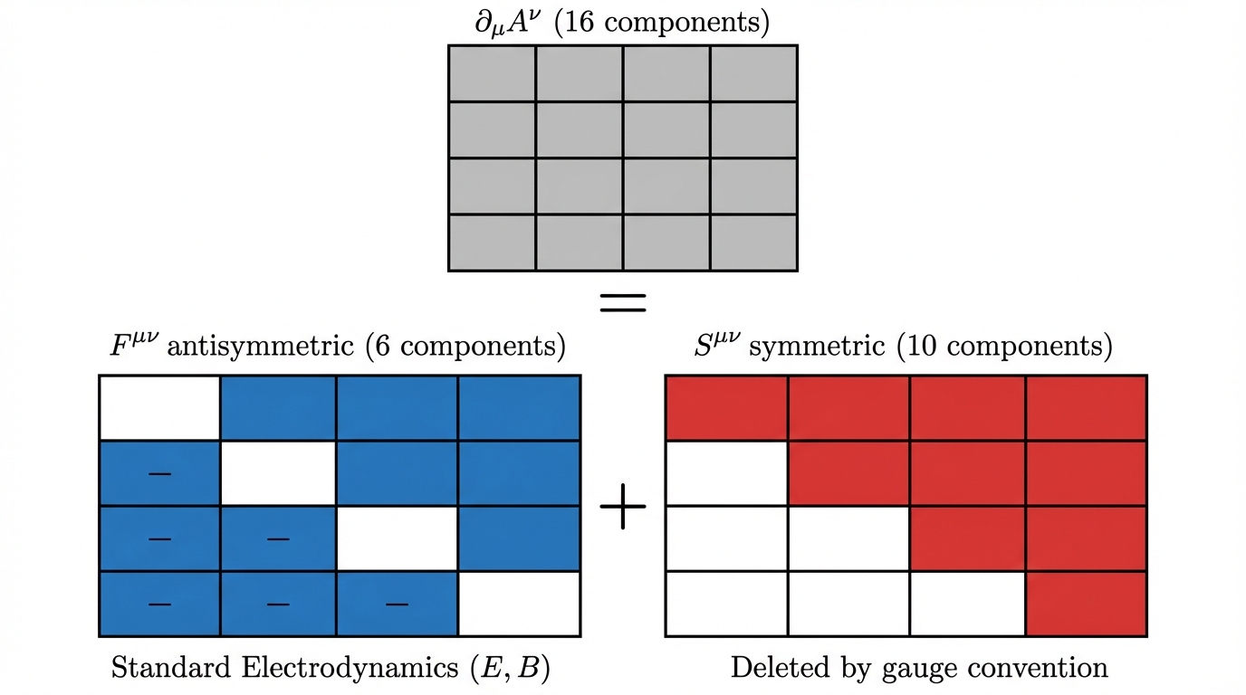
The answer is substantial. The full four-gradient \(\partial_\mu A_\nu\) has 16 independent kinematic components; standard electrodynamics uses only the 6 antisymmetric ones. The remaining 10 — the symmetric part, including the scalar-longitudinal coupling that the Lorenz gauge sets to zero — are not proven absent. They are defined absent by the gauge convention.
2 The Full Potential Tensor
Before examining the historical construction of the field-primary convention and the physical content it removed, it is necessary to establish the mathematical framework that makes precise what was deleted. The standard formulation of electrodynamics uses only part of the information contained in the electromagnetic potentials. This section exhibits the full structure and identifies exactly which parts each gauge convention discards.
2.1 Maxwell’s Seventh Component
Maxwell’s original formulation [3] used quaternion algebra, in which the nabla operator acting on a quaternion-valued potential produces a full quaternion with both scalar and vector parts (Eq. (5)). The vector part gives the magnetic field \(\mathbf{B} = \nabla \times \mathbf{A}\). The scalar part defines a seventh field component:
\[T = -\frac{1}{c}\frac{\partial \phi}{\partial t} + \nabla \cdot \mathbf{A} \tag{1}\label{eq:T-component}\]
This is not an exotic quantity. It is the scalar part of the quaternion electric field, produced by the same algebraic operation that yields \(\mathbf{E}\) and \(\mathbf{B}\). In Hamilton’s quaternion calculus, the nabla-potential product is a single indivisible operation; \(T\) and \(\mathbf{B}\) are co-equal outputs. Heaviside and Gibbs split this product into two independent operations (divergence and curl) and then suppressed \(T\) — not because it was shown to be unphysical, but because it complicated the equations.
The Lorenz gauge condition (Eq. (6)) is precisely the statement \(T = 0\). Setting the trace to zero is a postulate, not a discovery — a choice to discard a dynamical variable. When Reed and Hively [4] developed Extended Electrodynamics by relaxing the Lorenz gauge, what they recovered (their scalar field \(C\), Eq. (12)) is Maxwell’s \(T\) component under a different name and a different unit convention.
The notational relationship between \(T\) and \(C\) deserves explicit clarification to avoid confusion. Maxwell’s seventh component (Eq. (1)) is defined as \(T = -(1/c)\,\partial_t\phi + \nabla\cdot\mathbf{A}\), where the factor \(1/c\) arises from the quaternion convention in which the timelike component of the potential is \(\phi/c\). The EED scalar field (Eq. (12)) is defined as the Lorenz four-divergence \(C = \partial_\mu A^\mu = \nabla\cdot\mathbf{A} + (1/c^2)\,\partial_t\phi\), where the factor \(1/c^2\) arises from the SI convention for the d’Alembertian acting on \(A_0 = \phi/c\). The two are related by \(T = -cC\): they differ by a sign (opposite convention for which term carries the minus sign) and a factor of \(c\) (dimensional conversion between the two representations). Both vanish under the Lorenz gauge, and both become dynamical fields when the gauge is relaxed. Throughout this paper, \(C\) denotes the Lorenz divergence in the SI convention of Eq. (12).
2.2 The 16-Component Decomposition
The mathematical content of the deletion becomes precise in tensor language. The four-gradient of the four-potential \(A_\nu = (\phi/c,\, \mathbf{A})\) is a rank-2 tensor with 16 independent components:
\[\partial_\mu A_\nu = \underbrace{\frac{1}{2}(\partial_\mu A_\nu - \partial_\nu A_\mu)}_{F_{\mu\nu}\;\text{(antisymmetric, 6 components)}} + \underbrace{\frac{1}{2}(\partial_\mu A_\nu + \partial_\nu A_\mu)}_{S_{\mu\nu}\;\text{(symmetric, 10 components)}} \tag{2}\label{eq:16-decomp}\]
The antisymmetric part \(F_{\mu\nu}\) is the electromagnetic field tensor, encoding \(\mathbf{E}\) and \(\mathbf{B}\) in its six independent components. This is the only part that standard electrodynamics retains.
The symmetric part \(S_{\mu\nu}\) has ten independent components. Its trace is:
\[S^\mu{}_\mu = \partial_\mu A^\mu = \frac{1}{c}\frac{\partial \phi}{\partial t} + \nabla \cdot \mathbf{A} \tag{3}\label{eq:S-trace}\]
which is (up to sign) Maxwell’s \(T\) component. The Lorenz gauge sets this trace to zero.
Standard electrodynamics uses 6 of the 16 kinematic components. The remaining 10 are not proven absent. They are defined absent by the gauge convention.
A precise distinction is necessary, and it is the distinction between kinematic components and dynamical degrees of freedom. The 16-component decomposition of \(\partial_\mu A_\nu\) is kinematic: it identifies the mathematical content available in the tensor. But the number of propagating degrees of freedom is a separate, dynamical question — one that requires a Lagrangian and constraint analysis to answer.
The underlying field is \(A_\mu\): four components, not sixteen. The tensor \(\partial_\mu A_\nu\) is a derived object — sixteen functions of four fields. Just as the symmetric metric perturbation \(h_{\mu\nu}\) in linearized general relativity has ten independent components but only two propagating degrees of freedom (the transverse-traceless polarizations, with the remainder eliminated by diffeomorphism gauge and constraint equations), the symmetric part \(S_{\mu\nu}\) has ten kinematic components but cannot support ten independent propagating modes. The four-potential \(A_\mu\) allows at most \(4 - 1 = 3\) propagating degrees of freedom: four field components minus one gauge parameter. In standard electrodynamics (Lorenz gauge imposed), the Gauss constraint further reduces this to \(3 - 1 = 2\) — the two transverse polarizations. In Extended Electrodynamics (Section 4.3), where the Lorenz gauge is relaxed and the gauge-fixing term is promoted to a dynamical term (\(\gamma = 1\) in the Stueckelberg Lagrangian), all three modes propagate: two transverse and one scalar-longitudinal, the latter being the field \(C\) (Eq. (12)).
The kinematic and dynamical perspectives are complementary, not contradictory. The 16-component decomposition shows what information the four-gradient carries. The Lagrangian analysis shows which part propagates. Of the ten symmetric components, the trace constitutes the one new propagating mode that EED recovers; the nine traceless components are not independent fields but kinematic functions of the same four-component \(A_\mu\) that already determines the six antisymmetric components. The “deletion” performed by gauge fixing is real — it discards kinematic information from \(\partial_\mu A_\nu\) that EED retains — but it is a deletion of one dynamical mode, not ten.
The gauge dependence of \(S_{\mu\nu}\) requires the same care. Under a gauge transformation \(A_\mu \to A_\mu + \partial_\mu\chi\), the symmetric part transforms as \(S_{\mu\nu} \to S_{\mu\nu} + \partial_\mu\partial_\nu\chi\). This means \(S_{\mu\nu}\) is gauge-dependent — but the same is true of \(A_\mu\) itself, and the Aharonov-Bohm effect (Section 4.1) demonstrates that gauge-dependent quantities can carry gauge-invariant physical content. The template is the same: \(A_\mu\) is gauge-dependent, but its holonomy \(\oint A_\mu\, dx^\mu\) is gauge-invariant. Similarly, \(S_{\mu\nu}\) is gauge-dependent, but in the EED framework (\(\gamma = 1\)), its trace \(\partial_\mu A^\mu\) is promoted to a dynamical field \(C\) with its own equation of motion — and the dynamics of \(C\) are physical because the theory is gauge-free by construction. There is no residual gauge transformation available to remove \(C\); the Stueckelberg parameter \(\gamma = 1\) has eliminated the gauge freedom that would otherwise allow it.
2.3 The Helmholtz Decomposition in Four Dimensions
The three-dimensional Helmholtz decomposition [5] splits any vector field into irrotational (curl-free) and solenoidal (divergence-free) parts. Extended to four dimensions via the Hodge decomposition, the antisymmetric and symmetric parts of \(\partial_\mu A_\nu\) acquire geometric meaning:
The antisymmetric part \(F_{\mu\nu}\) (a 2-form) encodes the solenoidal, transverse sector — electromagnetic waves, radiation, and the phenomena that standard electrodynamics describes exactly.
The symmetric part \(S_{\mu\nu}\) encodes the irrotational, longitudinal sector — scalar-longitudinal coupling, force-free potentials, and phenomena that produce longitudinal \(\mathbf{E}\) without \(\mathbf{B}\). In the language of the Hodge decomposition, \(S_{\mu\nu}\) contains the exact and harmonic parts that the 2-form \(F_{\mu\nu}\) cannot represent.
The Hodge decomposition adds a further insight absent from the three-dimensional case: the harmonic component, which is topologically conserved and carries information about the global structure of the space (winding numbers, cohomology classes). This harmonic part is precisely what gauge-invariant quantities like the Aharonov-Bohm phase and magnetic helicity encode (Section 4.1).
2.4 What Each Gauge Kills
Different gauge choices eliminate different subsets of the 10 symmetric components:
| Gauge | Condition | Physical content eliminated |
|---|---|---|
| Lorenz | \(\partial_\mu A^\mu = 0\) | Trace of \(S_{\mu\nu}\); scalar field \(T\); decouples \(\phi\) from \(\mathbf{A}\); forces advanced and retarded potentials to separate |
| Coulomb | \(\nabla \cdot \mathbf{A} = 0\) | All longitudinal components of \(\mathbf{A}\); no elasticity, no longitudinal waves; \(\phi\) becomes instantaneous |
| Temporal | \(A_0 = 0\) (\(\phi = 0\)) | Scalar potential; electric field becomes purely inductive; static electric phenomena require special treatment |
| Axial | \(A_3 = 0\) | One spatial component; breaks manifest Lorentz covariance; hides polarization information |
The critical observation is that every gauge choice is a projection from the full 16-component tensor onto a reduced subspace. The projection simplifies computation at the cost of discarding information. The question this paper asks is not whether these projections are mathematically valid — they are — but whether the discarded information has physical content.
2.5 The Geometric Algebra Perspective
Hestenes’ spacetime algebra (STA) [6], [7] provides a modern resolution of the quaternion structure that Heaviside dismantled. In STA, the geometric product of the nabla operator with the vector potential naturally unifies the divergence and curl:
\[\nabla A = \nabla \cdot A + \nabla \wedge A \tag{4}\label{eq:sta-product}\]
where \(\nabla \wedge A\) is the exterior (wedge) product giving the bivector field \(F\) (the electromagnetic field), and \(\nabla \cdot A\) is the inner product giving the scalar field. In geometric algebra, these are not two separate operations applied independently — they are the two grades of a single geometric product, inseparable by construction.
This makes the Heaviside truncation algebraically visible: separating curl from divergence and discarding the scalar part is equivalent to projecting out one grade of a multivector. The full geometric product \(\nabla A\) recovers the complete information content of \(\partial_\mu A_\nu\) in a form that treats all components on equal algebraic footing. The scalar part was never optional in the algebra. It was half of a single operation.
3 Three Acts of Deletion
The ontological demotion of potentials was not a discovery. It was constructed through three deliberate choices, each of which traded physical content for mathematical convenience.
3.1 Act 1: Heaviside’s Vector Reduction (1880s)
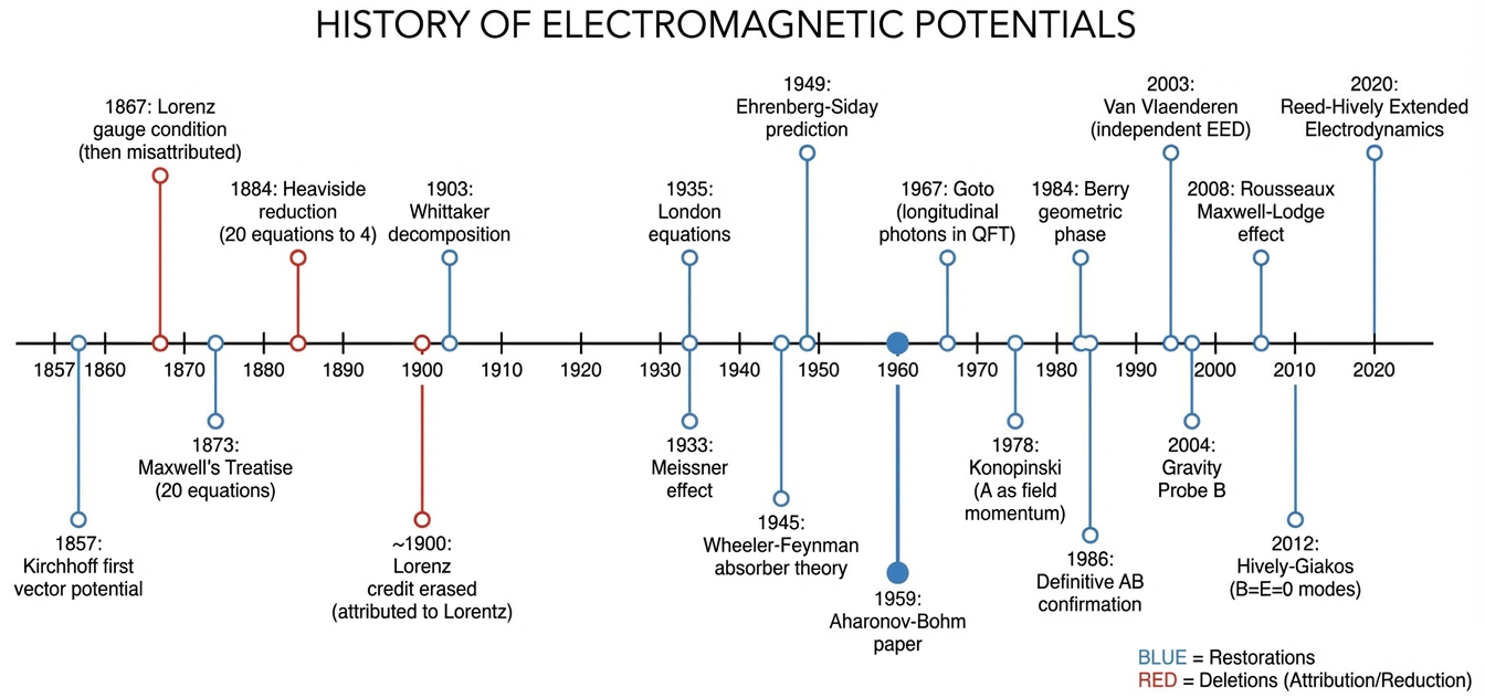
Maxwell’s original formulation [3] used quaternions and contained twenty equations in twenty unknowns, expressing the full structure of electromagnetic phenomena including potentials as central objects. Maxwell treated the vector potential as a primary physical quantity, calling it “electromagnetic momentum” — a term implying physical reality, not mathematical convenience. Between 1882 and 1884, Heaviside [2] reformulated this using vector calculus, reducing twenty equations to the four taught today.
This was a triumph of mathematical economy. It was also a deletion. The specific content that was lost can be exhibited concretely. In Hamilton’s quaternion calculus, when the nabla operator acts on the vector potential \(\mathbf{A}\), the result is a full quaternion with both scalar and vector parts [3]:
\[\nabla \mathbf{A} = \underbrace{-\nabla \cdot \mathbf{A}}_{\text{scalar part}} + \underbrace{\nabla \times \mathbf{A}}_{\text{vector part}} \tag{5}\label{eq:quaternion-product}\]
The vector part gives the magnetic field: \(\nabla \times \mathbf{A} = \mathbf{B}\). The scalar part, \(-\nabla \cdot \mathbf{A}\), has no counterpart in the modern four equations. In Maxwell’s framework, these two parts are produced by a single algebraic operation — they are inseparable components of one quaternion quantity. Heaviside and Gibbs split them into two independent operations (dot product and cross product) and then physically suppressed the scalar part by either setting \(\nabla \cdot \mathbf{A} = 0\) (Coulomb gauge) or constraining it via the Lorenz condition (Eq. (6)) [2].
Heaviside was explicit about his intent: he found potentials “mystical” and sought to “murder them from the theory” [2]. In a letter to Oliver Lodge, he claimed his reformulation represented “the real and true Maxwell” as Maxwell would have written it had he not been “humbugged by his vector and scalar potentials” [2]. Hertz went further, declaring potentials “not physical magnitudes” but useful “for calculations only” [8]. Gibbs acknowledged the trade-off: the scalar and vector parts “represented important operations, but their union … did not seem a valuable idea” [9]. The elimination was not a unified program but an accidental consensus: Heaviside wanted to keep scalar potentials while eliminating vector potentials; Hertz preferred to eliminate both [8]. What survived was neither man’s preference but a compromise that stripped all potentials of physical status.
The consequences are concrete. Setting \(\nabla \cdot \mathbf{A} = 0\) eliminates the scalar-longitudinal coupling between \(\nabla \cdot \mathbf{A}\) and \(\partial \phi / \partial t\) — precisely the coupling that Extended Electrodynamics (Section 4.3) recovers as the dynamical scalar field \(C\) (Eq. (12)). Restoring what Heaviside set to zero does not modify any transverse prediction of standard electrodynamics. It adds a longitudinal sector that the standard theory structurally cannot represent.
The pragmatic counterargument is strong: Heaviside’s simplification works. The four vector equations predict every phenomenon that 19th-century physics could measure, and the transverse sector they describe remains the foundation of electrical engineering, antenna theory, and photonics. The deletion was not wrong in any practical sense for the physics of the time. It was incomplete — and the incompleteness became visible only when quantum mechanics and gauge-free formulations revealed the physical content of what had been discarded.
The limitations of the replacement formalism reinforce the point. Gibbs and Heaviside’s vector calculus relies on the cross product, which exists only in three dimensions [9]. In four-dimensional spacetime, there is no unique perpendicular direction, and the cross product has no natural extension. The quaternion product that Maxwell used has no such limitation: it operates in any dimension because it encodes both symmetric (inner) and antisymmetric (outer) products simultaneously. The four-dimensional Heaviside-Gibbs formalism works only by importing the exterior algebra of differential forms — which is, mathematically, the quaternion structure under a different name.
Jefimenko [10] sharpened the critique from a different angle: \(\mathbf{E}\) and \(\mathbf{B}\) do not cause each other. The standard narrative of electromagnetic induction — a changing \(\mathbf{B}\) “produces” \(\mathbf{E}\), and vice versa — is pedagogically convenient but physically incorrect. Both fields are independently caused by charges and currents. Their time derivatives happen to satisfy coupled equations, but the causal chain runs from sources to fields, not from field to field. This undermines the conceptual foundation of the field-primary hierarchy: if \(\mathbf{E}\) and \(\mathbf{B}\) are not even causally primary with respect to each other, elevating them above the potentials from which they derive is doubly unjustified.
3.2 Act 2: The Lorenz Gauge Convention
The Lorenz gauge condition (due to the Danish physicist Ludvig Lorenz [11], not the Dutch physicist Hendrik Lorentz) imposes:
\[\nabla \cdot \mathbf{A} + \frac{1}{c^2} \frac{\partial \phi}{\partial t} = 0 \tag{6}\label{eq:lorenz}\]
This decouples the wave equations for \(\phi\) and \(\mathbf{A}\), making them independently solvable. The mathematical simplification is significant. The physical cost is also significant: the gauge condition forces \(\nabla \cdot \mathbf{A}\) to be determined entirely by \(\partial \phi / \partial t\). Any independent physical content carried by \(\nabla \cdot \mathbf{A}\) is suppressed.
The misattribution is itself revealing. Lorenz derived retarded potentials and the gauge condition in 1867 [11], but Maxwell publicly objected to the retarded-potential approach in 1868, arguing it violated energy conservation [8]. Coming from Maxwell’s authority, this critique was devastating to Lorenz’s recognition. By 1900, Wiechert had erased Lorenz from the citation chain entirely, and des Coudres referred to retarded solutions as “Lorentz’sche Lösungen.” The condition that should bear Lorenz’s name was cemented under Lorentz’s within a single generation — a case study in how social dynamics, not scientific priority, shape the narrative of physics [8].
The Lorenz gauge also constrains the temporal structure of the theory. The general solution to the wave equation admits both retarded and advanced potentials. Standard practice discards the advanced solutions as “unphysical.” Wheeler and Feynman [12], [13] showed this is not required by the theory. Their absorber theory demonstrated that a time-symmetric formulation using equal parts retarded and advanced potentials is fully consistent with observed phenomena. The apparent arrow of time in radiation emerges from boundary conditions, not from a fundamental asymmetry in the equations. Advanced solutions carry physical content about absorber boundary conditions that the retarded-only formulation discards.
The 16-component decomposition of Section 2.2 makes the cost precise. In the Lorenz gauge, the trace of \(S_{\mu\nu}\) (Eq. (3)) vanishes, eliminating the scalar field \(T\). In the Coulomb gauge (\(\nabla \cdot \mathbf{A} = 0\)), all longitudinal components of \(\mathbf{A}\) vanish — the vector potential has zero elasticity, carries no longitudinal information, and \(\phi\) becomes an instantaneous (non-retarded) quantity. Different gauges project onto different 6-dimensional subspaces of the full 16-dimensional space, and each projection discards different physics. The fact that all gauges agree on the transverse sector is precisely the statement that all gauges agree on \(F_{\mu\nu}\) — the 6-component antisymmetric part. They disagree about \(S_{\mu\nu}\) — the 10 components that no gauge retains in full.
3.3 Act 3: The Ontological Demotion
The first two acts removed specific mathematical terms. The third act was philosophical: the consensus that gauge freedom proves potentials are unphysical. If \(\mathbf{A}\) can be transformed as \(\mathbf{A} \to \mathbf{A} + \nabla\chi\) without changing observables, the argument goes, then \(\mathbf{A}\) cannot be physical.
But the Aharonov-Bohm phase (Eq. (7)) is gauge-invariant. The London equation (Eq. (8)) fixes \(\mathbf{A}\) physically in a superconductor. Gauge freedom constrains the description of \(\mathbf{A}\), not its ontological status. The argument from gauge freedom proves only that \(\mathbf{A}\) contains more information than any single gauge-fixed representation captures — which is an argument for its richness, not its unreality.
3.4 The Combined Effect
Heaviside’s reduction eliminated longitudinal modes and scalar-vector coupling. The Lorenz gauge eliminated the independent content of \(\nabla \cdot \mathbf{A}\) and advanced solutions. The ontological demotion eliminated the motivation to investigate what had been removed. Together, they narrowed the theory from a rich potential-primary framework to a field-primary one with fewer degrees of freedom.
Neither simplification was wrong in the sense of producing incorrect predictions for the phenomena known at the time. Both were wrong in the sense of promoting a contingent mathematical choice to the status of physical truth — a promotion that every subsequent experimental test has contradicted.
4 The Deleted Physics
The three acts of deletion did not merely change notation. They removed physical content that can be precisely identified. This section presents each deleted sector together with the evidence that establishes its physical reality. The evidence spans five domains: topological structure (Section 4.1), condensed matter physics (Section 4.2), the scalar-longitudinal sector and its consequences for forces and energy flow (Sections 4.3–4.6), the potential hierarchy, quantum persistence, and time symmetry (Sections 4.7–4.8 and the following section), and the connections to gravitation and the quantum vacuum (Sections 4.10–4.11). Their convergence from independent lines of inquiry is the argument.
4.1 Topological Structure and the Aharonov-Bohm Effect
The deepest argument for potential primacy is topological. In the fiber bundle formulation of gauge theory [14], the electromagnetic potential \(A_\mu\) is a connection on a principal \(U(1)\) bundle over spacetime, and the field tensor \(F_{\mu\nu}\) is its curvature. This is not a metaphor. It is the mathematical structure that the Standard Model uses.
The critical insight is that connections carry more information than curvatures. A flat connection (\(F_{\mu\nu} = 0\) everywhere) can still have non-trivial holonomy — a non-zero phase acquired by parallel transport around a closed loop — if the base space has non-trivial topology. Holonomy is a geometric property of the connection. It does not require quantization, \(\hbar\), or wave mechanics. The curvature tells you the local geometry; the connection tells you the global topology. Gauge fixing, by projecting the connection onto a specific section of the bundle, can destroy this global information.
The Aharonov-Bohm effect is the physical manifestation of this mathematical fact. First noted by Ehrenberg and Siday [15] and formalized by Aharonov and Bohm [16] (AB), a charged particle traversing a region where \(\mathbf{B} = 0\) but \(\mathbf{A} \neq 0\) acquires a measurable phase shift: \[\Delta\varphi = \frac{e}{\hbar} \oint \mathbf{A} \cdot d\mathbf{l} \tag{7}\label{eq:ab-phase}\]
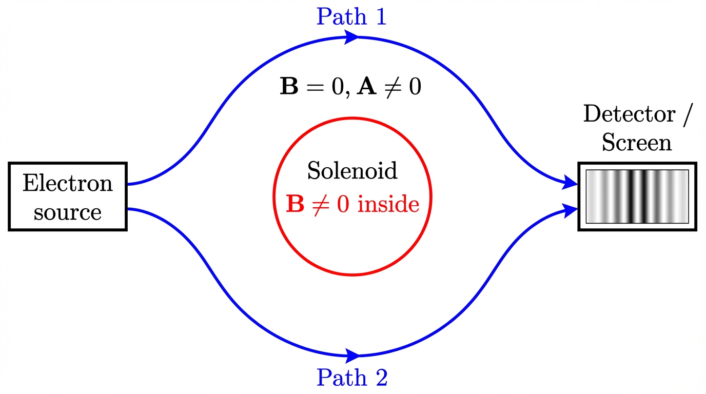
The experimental confirmation progressed through three decades of increasing precision. Chambers [17] provided the first observation using an iron whisker, though field leakage remained a concern. Tonomura [18] used electron holography with nanoscale toroidal ferromagnets, confining flux within closed loops. The definitive confirmation by Osakabe et al. [1] enclosed a toroidal magnet in a superconducting niobium shell, where the Meissner effect [19] guaranteed complete confinement of \(\mathbf{B}\). The phase sensitivity reached \(2\pi/100\), and the shift of \(\pi\) for half-integer flux quanta left no alternative explanation. The electrons never encounter \(\mathbf{B}\). They encounter \(\mathbf{A}\).
The Aharonov-Bohm effect is routinely classified as a quantum phenomenon. This classification obscures the point just established: the phase shift of Eq. (7) is the holonomy of the \(U(1)\) connection — a geometric property that exists independently of quantum mechanics. The AB effect is not a quantum correction to classical electrodynamics. It is a topological property of the connection that becomes observable through quantum interference but exists at all scales. If the AB effect were purely quantum, one could argue that the deleted degrees of freedom are relevant only at quantum scales. But the connection formulation shows that potentials carry topological information — holonomy, monodromy, winding numbers — at all scales. The deletion did not remove quantum corrections. It removed geometric structure.
The principle extends beyond the solenoid geometry and beyond the quantum scale. The Maxwell-Lodge effect [20] provides a purely classical demonstration: Lodge wound a primary coil on a toroidal solenoid and detected induced voltage in a secondary coil outside the torus, where \(\mathbf{B} = 0\). Rousseaux et al. confirmed the result with modern instrumentation, measuring a voltage governed by \(\mathbf{E} = -\partial\mathbf{A}/\partial t\) in a region of strictly zero magnetic field. The harmonic component of \(\mathbf{A}\) — simultaneously divergence-free and curl-free — propagates electromagnetic influence classically, without quantum interference or \(\hbar\). This is the Aharonov-Bohm effect at macroscopic scale, in the laboratory of Faraday induction.
Konopinski [21] sharpened the theoretical argument by re-expressing the equation of motion in terms of canonical momentum: \(\mathbf{p} = m\mathbf{v} + q\mathbf{A}/c\). A charged bead sliding on a circular fiber concentric with a solenoid experiences a velocity change when the solenoid current varies — the change in \(\mathbf{A}\) produces a compensating change in kinetic momentum \(m\mathbf{v}\) through canonical momentum conservation. Monitoring the bead’s velocity change at every point directly measures \(\mathbf{A}\). The vector potential is not a mathematical abstraction. It is Faraday’s “electrotonic state” — a store of field momentum available for exchange with charged particles.
The argument extends from theory to engineering practice. Reed [22] reviewed the Vector Potential Transformer (VPT) developed by Daibo et al., a patented device using a “coiled coil” geometry — a flexible solenoid wound toroidally, with its return wire running coaxially through the core. This geometry ensures \(\mathbf{B} = 0\) everywhere outside the primary winding while maintaining a non-zero \(\mathbf{A}\). A secondary toroidal coil placed in the field-free region detects an induced voltage governed by \(-\partial\mathbf{A}/\partial t\). The VPT penetrates conductive shields that block all conventional electromagnetic signals — voltage appears even when the secondary is enclosed in conducting material. Applications include sensing through reactor pressure vessels, deep-sea water, and biological tissue.
The counterargument — that near-field capacitive or inductive coupling could explain shield penetration without invoking \(\mathbf{A}\) directly — does not survive the geometry: the VPT’s coiled-coil topology produces strictly \(\mathbf{B} = 0\) outside the primary, and the secondary voltage’s path dependence is a signature of the harmonic component of \(\mathbf{A}\), not of stray fields. The vector potential is not merely “real enough” to shift quantum phases. It is real enough to build patented industrial devices on.
Any configuration that produces \(\mathbf{E} = 0\), \(\mathbf{B} = 0\) while maintaining \(\mathbf{A} \neq 0\) or \(\phi \neq 0\) demonstrates potential primacy. Such compensated configurations can be achieved systematically: when counter-wound conductors cancel their fields everywhere outside the winding region, the vector potential remains non-zero and extends into the field-free region. The principle extends to the electric side: when a capacitive element is wound on a surface with non-trivial topology, the resulting scalar potential \(\phi\) can become multi-valued, demonstrating that the topological richness of potentials is not limited to \(\mathbf{A}\) and the magnetic sector.
Berry’s geometric phase [23] generalizes this to any quantum system undergoing adiabatic cyclic evolution. The Aharonov-Bohm phase is the special case where \(\mathbf{A}\) serves as the connection. This points to the general principle that the gauge-theoretic formulation of the Standard Model already implements: the fundamental quantities in physics are connections (potentials), not curvatures (fields). Feynman, after presenting the Aharonov-Bohm effect in the Lectures on Physics, concluded that “in our sense then, the \(A\)-field is ‘real’ ” [24] — a notable concession from a physicist who had originally approached electrodynamics through fields.
The argument extends to both components of the four-potential. Aharonov and Bohm’s original paper [16] proposed a dual effect involving the scalar potential \(\phi\): a charged particle traversing a field-free region of nonzero \(\phi\) acquires a phase shift \(\Delta\varphi = (q/\hbar)\int \phi\, dt\), depending solely on the time integral of the potential experienced. The electric AB effect awaits clean experimental confirmation — the difficulty is practical, requiring potential switching faster than the electron’s transit time — but its theoretical basis is identical to the magnetic case. Together, both effects demonstrate that the full electromagnetic four-potential \(A^\mu = (\phi/c,\, \mathbf{A})\), not merely one component of it, constitutes the physically fundamental quantity, with each component independently producing observable consequences in field-free regions.
Magnetic helicity [25], [26] provides a concrete example of topological information carried by potentials. Defined as \(\mathcal{H} = \int \mathbf{A} \cdot \mathbf{B}\, d^3x\), it measures the topological linkage and knottedness of magnetic field lines. Despite being defined in terms of the gauge-dependent \(\mathbf{A}\), magnetic helicity is gauge-invariant for closed magnetic field configurations. It is a conserved quantity in ideal magnetohydrodynamics and determines the minimum-energy configurations into which turbulent plasmas relax [27]. Taylor relaxation — the self-organization of turbulent plasma into discrete topological states labeled by winding numbers — is “classical quantization from topology”: discrete states emerging from a conserved topological invariant without any role for \(\hbar\).
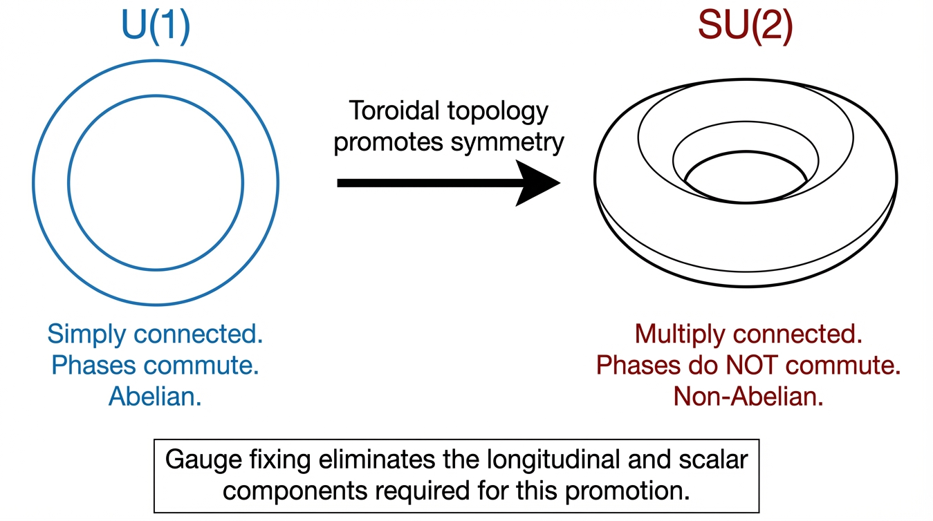
The gauge-theoretic structure extends beyond \(U(1)\). Barrett [14] argued that toroidal geometries can promote the symmetry group from \(U(1)\) to \(SU(2)\), generating non-Abelian phase factors — phase-dependent quantities that do not commute under composition. (Barrett’s specific mathematical execution has been critiqued [28] as insufficiently rigorous; this paper does not endorse Barrett’s formalism. The underlying topological principle, however, is independent of Barrett’s execution: the Wu-Yang nonintegrable phase factor framework and the multiply connected topology of the torus are established mathematical results that permit non-Abelian holonomies without requiring Barrett’s construction.) In the \(U(1)\) case, the order of phase accumulations does not matter. In the \(SU(2)\) case, the path through configuration space determines the outcome. This non-commutativity is a direct consequence of the topological richness of the potential and has no representation in terms of \(\mathbf{E}\) and \(\mathbf{B}\) alone. The promotion from \(U(1)\) to \(SU(2)\) requires precisely the longitudinal and scalar potential components that gauge fixing eliminates.
The topological argument makes the strongest case against the claim that potentials are “merely mathematical.” The topology of the connection — its holonomy group, its characteristic classes, its monodromy — is physical, measurable, and irreducible to field quantities. Gauge fixing does not remove “unphysical redundancy.” It projects out topological information that the fields cannot reconstruct.
4.2 Superconductor Physics: Potential Primacy in the Laboratory
The second London equation [29] provides what may be the most direct engineering evidence for potential primacy:
\[\mathbf{J}_s = -\frac{n_s e^2}{m} \mathbf{A} \tag{8}\label{eq:london2}\]
In the London gauge (\(\nabla \cdot \mathbf{A} = 0\), physically enforced by the superconductor’s response), the supercurrent is directly proportional to the vector potential — not to \(\mathbf{E}\), not to \(\mathbf{B}\), but to \(\mathbf{A}\) itself. One might object that this form is gauge-dependent. But that is precisely the point: the superconductor selects a gauge physically, through the Meissner effect, rather than mathematically. Nature fixes \(\mathbf{A}\) where textbooks say it is arbitrary. This is the operating principle of every superconducting device: SQUIDs, MRI magnets, particle accelerators. Engineering already uses \(\mathbf{A}\) as the primary variable and has done so since 1935. The field-primary formulation persists in textbooks while the laboratories moved on decades ago. Flux quantization reinforces the point. London predicted [30] that magnetic flux through a superconducting ring is quantized:
\[\oint \mathbf{A} \cdot d\mathbf{l} = n \frac{h}{2e}, \quad n \in \mathbb{Z} \tag{9}\label{eq:flux-quant}\]
The fundamental constraint acts on \(\mathbf{A}\), not on \(\mathbf{B}\). The vector potential’s role extends beyond superconductors into normal metals. Büttiker, Imry, and Landauer [31] predicted that mesoscopic normal-metal rings — small enough for electron phase coherence to span the circumference — carry equilibrium persistent currents that oscillate with the Aharonov-Bohm period \(h/e\) as a function of the enclosed magnetic flux. Lévy et al. [32] confirmed this experimentally in copper rings. Unlike interference-fringe experiments, persistent currents demonstrate that the vector potential \(\mathbf{A}\) governs the ground-state energy spectrum of a many-body quantum system, establishing its role as a thermodynamically consequential quantity rather than a gauge-dependent auxiliary.
The superconductor’s role extends beyond demonstrating that \(\mathbf{A}\) is physical: Li and Torr showed that the same condensate may simultaneously fix the gravitational vector potential (Section 4.10), and Mead connected flux quantization to the potential hierarchy through the superpotential (Section 4.7). The superconductor is not merely evidence for potential primacy — it is the laboratory where potential primacy has been engineering practice for nine decades.
4.3 The Scalar-Longitudinal Sector
The recovery of the scalar-longitudinal sector has been achieved independently by multiple research programs spanning two decades, converging on the same physical content through different formalisms. Van Vlaenderen [33] derived the scalar field \(S = -\varepsilon_0\mu_0\,\partial\phi/\partial t - \nabla \cdot \mathbf{A}\) (the negative of the Lorenz condition) from first principles in 2003, showing that treating \(S\) as a dynamical field modifies Gauss’s law by a term \(-\partial S/\partial t\) and Ampère’s law by a term \(+\nabla S\). The modified Poynting vector becomes \(\mathbf{P} = \mathbf{E} \times \mathbf{B} - \mathbf{E}\,S\), introducing a scalar energy flux channel that operates independently of the magnetic field. Van Vlaenderen’s later work [34] extended this into General Classical Electrodynamics (GCED), predicting three independent wave types — transverse electromagnetic (TEM), longitudinal electromagnetic (LEM), and scalar (\(\Phi\)) waves — with potentially distinct phase velocities determined by new vacuum constants. Hively and Giakos [35] arrived at the same scalar field (denoted \(\xi\)) via the four-vector wave equation, identifying five new wave solutions with \(\mathbf{B} = \mathbf{E} = 0\) — pure scalar modes carrying energy but no momentum, driven by irrotational (gradient) currents. The convergence of these independent programs is summarized in Table 2.
| Authors | Year | Formalism | Scalar field |
|---|---|---|---|
| Van Vlaenderen | 2003 | Helmholtz decomposition | \(S\) |
| Hively & Giakos | 2012 | Four-vector wave equation | \(\xi\) |
| Van Vlaenderen | 2016 | GCED (three wave types) | \(S\) |
| Reed & Hively | 2020 | Stueckelberg Lagrangian | \(C\) |
Reed and Hively [4] synthesized these threads into Extended Electrodynamics (EED), a gauge-free formulation whose Lagrangian derives from the Stueckelberg mechanism [36] — the same framework used in gauge-invariant massive electrodynamics. Woodside [37] proved uniqueness theorems for three-vector and scalar field decompositions in Minkowski space, showing that the four-potential decomposes into exactly two physically distinct classes: the four-solenoidal class (zero four-divergence, recovering standard electrodynamics under the Lorenz gauge) and the four-irrotational class (zero four-curl, \(F_{\mu\nu} = 0\)), which is the scalar-longitudinal sector. These theorems establish EED as the provably unique gauge-free extension of Maxwell’s equations when the Lorenz gauge constraint is relaxed.
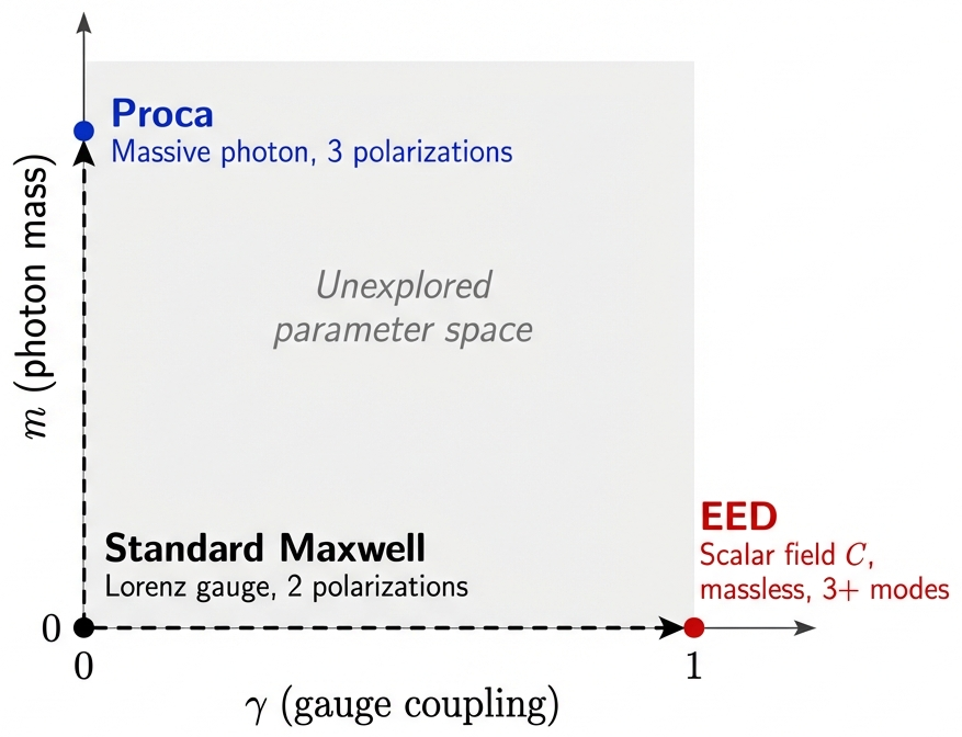
The Stueckelberg Lagrangian provides a unified view. In its general form, the Lagrangian density reads [4], [36]: \[\mathcal{L} = -\frac{1}{4}F_{\mu\nu}F^{\mu\nu} + \frac{\gamma}{2}(\partial_\mu A^\mu)^2 - \frac{1}{2}m^2 A_\mu A^\mu - J_\mu A^\mu \tag{10}\label{eq:eed-lagrangian}\] The first term is the standard Maxwell Lagrangian. The second term, proportional to \(\gamma\), is the key: when \(\gamma = 0\), this term vanishes and the Lorenz gauge can be imposed as an external constraint. When \(\gamma = 1\), this term becomes a kinetic contribution for the scalar field \(C = \partial_\mu A^\mu\), giving it dynamical content. The third term is the Proca mass term, and \(J_\mu\) is the four-current source. The Euler-Lagrange equations of Eq. (10) yield: \[\partial_\nu F^{\mu\nu} + \gamma\,\partial^\mu(\partial_\nu A^\nu) - m^2 A^\mu = J^\mu \tag{11}\label{eq:eed-eom}\] For \(\gamma = 0\), \(m = 0\): the standard Maxwell equations. For \(\gamma = 1\), \(m = 0\): taking the four-divergence of Eq. (11) and using the antisymmetry of \(F^{\mu\nu}\) (which gives \(\partial_\mu\partial_\nu F^{\mu\nu} = 0\) identically) yields \(\Box C = \partial_\mu J^\mu\) — the scalar field \(C\) satisfies a wave equation sourced by charge non-conservation. For conserved currents (\(\partial_\mu J^\mu = 0\)), this becomes the free wave equation \(\Box C = 0\): the scalar field propagates at the speed of light as a free field. Two parameters — mass \(m\) and gauge-coupling constant \(\gamma\) — span the full space of theories (Table 3).
| Theory | \(\boldsymbol{\gamma}\) | \(\boldsymbol{m}\) | Longitudinal sector |
|---|---|---|---|
| Standard Maxwell (Lorenz gauge) | 0 | 0 | Absent (gauge-fixed away) |
| Proca (massive photon) | 0 | \(>0\) | 3rd polarization via mass |
| EED (gauge-free, massless) | 1 | 0 | Scalar field \(C\) |
4.4 Scalar-Longitudinal Signatures
The convergence of independent derivations establishes the theoretical foundation. What observable signatures would the scalar-longitudinal sector produce? EED provides specific, testable predictions centered on a scalar field \(C\) defined by:
\[C = \nabla \cdot \mathbf{A} + \frac{1}{c^2} \frac{\partial \phi}{\partial t} \tag{12}\label{eq:scalar-field}\]
In standard electrodynamics, the Lorenz gauge sets \(C = 0\) by convention. EED treats \(C\) as a dynamical field. The consequences are significant:
Ampere’s law gains a term \(-\nabla C\), and Gauss’s law gains a term \(\partial C / \partial t\). These terms affect only the irrotational (longitudinal) components — the solenoidal (transverse) electrodynamics of standard theory is unchanged.
EED predicts two new wave types: scalar-longitudinal waves (SLW), carrying both energy and momentum via a longitudinal \(\mathbf{E}\) field plus the scalar field \(C\); and free-space scalar waves (SW), carrying energy only.
Both SLW and SW are immune to the skin effect, since they carry no \(\mathbf{B}\) field. This is a testable, distinguishing prediction.
The EED Lagrangian (Eq. (10)) derives from Stueckelberg’s formulation and is provably unique [37].
The EED energy-momentum tensor, derived from the Lagrangian (Eq. (10)) via the standard Noether procedure, is conserved: \(\partial_\mu T^{\mu\nu} = 0\) in the absence of sources. The generalized Poynting vector \(\mathbf{P} = \mathbf{E}\times\mathbf{B} - \mathbf{E}\,C\) satisfies the continuity equation \(\partial u/\partial t + \nabla\cdot\mathbf{P} = 0\), where \(u = \frac{1}{2}(\mathbf{E}^2 + \mathbf{B}^2 + C^2)\) is the total field energy density including the scalar field contribution [4], [33]. Energy conservation is not broken by the additional sector; it is extended to include a scalar energy flux channel.
This is not speculative physics in the theoretical sense: it is the mathematically necessary consequence of not imposing the Lorenz gauge — of asking what happens when the content that Act 2 deleted is restored.
A concrete comparison illustrates the difference. Consider electromagnetic transmission through a conductive Faraday enclosure. In standard electrodynamics, the skin depth \(\delta = \sqrt{2/(\omega\mu\sigma)}\) determines attenuation: transverse electromagnetic waves, which carry \(\mathbf{B}\) fields, induce eddy currents that exponentially suppress transmission. A well-constructed Faraday cage blocks all standard EM signals.
EED predicts a qualitatively different outcome for scalar-longitudinal waves. Because SLW carry a longitudinal \(\mathbf{E}\) field and the scalar field \(C\) but no \(\mathbf{B}\) field [4], they do not induce the eddy currents responsible for skin-effect attenuation. EED therefore predicts that SLW penetrate Faraday enclosures — a testable signature with no explanation in standard electrodynamics. SLW are also predicted to exhibit \(1/r^2\) free-space attenuation (characteristic of scalar radiation) rather than \(1/r\) attenuation (characteristic of transverse radiation), and to be receivable by monopolar antennas that are insensitive to transverse waves.
Preliminary experimental results reported by Hively (US Patent 9,306,527 [38]) — including SLW transmission through Faraday enclosures, reception by monopolar antennas, and \(1/r^2\) free-space attenuation — are consistent with these predictions and cannot be explained by standard electrodynamics. These results have not been independently replicated, and the broader physics community treats them with appropriate caution given their extraordinary implications.
The strongest objection is immediate: quantum electrodynamics (QED), which does not include EED’s scalar field \(C\), is the most precisely tested theory in physics. Its predictions agree with experiment to better than one part in \(10^{12}\) (the electron magnetic moment anomaly). If the scalar-longitudinal sector were dynamically relevant, one might expect it to appear as a correction to QED precision tests. The EED response is that the scalar-longitudinal sector couples only to the irrotational (longitudinal) components of the field — precisely the components that QED’s transverse photon propagator does not probe. The two theories make identical predictions for all transverse phenomena. They diverge only for longitudinal configurations that standard experiments were not designed to test. Whether this divergence is real is an experimental question — one that the field-primary framework cannot even formulate.
A critical subtlety often missed in discussions of the scalar-longitudinal sector: the scalar potential \(\phi\) and the longitudinal component of \(\mathbf{A}\) do not propagate independently. They form a single coupled mode. The coupling term \(\nabla \cdot \mathbf{A} + (1/c^2) \partial\phi/\partial t\) entangles both potentials: \(\phi\) drives longitudinal \(\mathbf{A}\), and longitudinal \(\mathbf{A}\) drives \(\phi\). Together they propagate at \(c\) with a longitudinal \(\mathbf{E}\) field and no \(\mathbf{B}\) field. The propagation speed follows directly from the EED field equation (Eq. (11)): for \(\gamma = 1\) and \(m = 0\), the scalar field satisfies \(\Box C = 0\) in free space, where \(\Box = (1/c^2)\partial_t^2 - \nabla^2\) is the d’Alembertian. This is the standard wave equation with phase velocity and group velocity both equal to \(c\) — the same causal structure as transverse electromagnetic waves. No superluminal propagation arises; scalar-longitudinal waves respect the light cone. Separately, neither \(\phi\) nor \(A_L\) propagates at all.
This coupled nature explains why the scalar-longitudinal sector was invisible for so long: searching for “scalar waves” or “longitudinal \(\mathbf{A}\) waves” in isolation finds nothing. The mode exists only as a coupled \((\phi,\, A_L)\) entity — precisely the coupling that the Lorenz gauge destroys by freezing one in terms of the other.
The Proca equation [39] makes the connection between gauge freedom and the longitudinal sector explicit. For a massive vector boson, the Lagrangian includes a mass term \(\frac{1}{2}m^2 A_\mu A^\mu\) that breaks gauge invariance. The Proca field has three polarization states: two transverse (as in standard electrodynamics) and one longitudinal. The longitudinal polarization is not a theoretical curiosity — it is the mode that gives the \(W\) and \(Z\) bosons their third degree of freedom and makes the weak force short-ranged.
The Stueckelberg mechanism [36] restores gauge invariance to the massive theory by introducing a compensating scalar field \(\varphi_{\mathrm{S}}\) that absorbs the gauge variation of the mass term. The chain is: massless photon (2 polarizations, gauge-free) \(\to\) Proca (3 polarizations, gauge-broken) \(\to\) Stueckelberg (3 polarizations, gauge-restored via \(\varphi_{\mathrm{S}}\)). In unitary gauge (\(\varphi_{\mathrm{S}} = 0\)), the Stueckelberg theory reduces to Proca: the scalar field is “pure gauge” — it was introduced to be removed.
A natural objection follows: if the Stueckelberg scalar is pure gauge by construction, how can EED use the same mechanism to argue that the scalar field \(C\) is physical? The answer is that EED does not use the same mechanism. In the standard Stueckelberg theory (\(m > 0\)), the scalar compensates the gauge variation of the mass term. Its role is to restore a symmetry that the mass term broke. In EED (\(\gamma = 1\), \(m = 0\)), the scalar field \(C = \partial_\mu A^\mu\) is not a compensating field at all. It is the Lorenz divergence itself, promoted from a constraint (\(C = 0\) in the Lorenz gauge) to a dynamical variable (\(\Box C = \text{sources}\)). The gauge-fixing term in the standard Lagrangian — \((\gamma/2)(\partial_\mu A^\mu)^2\) — becomes a kinetic term when \(\gamma = 1\), and the resulting theory has no residual gauge symmetry. There is no unitary gauge available to remove \(C\), because there is no gauge freedom left to fix.
The distinction is between a scalar field introduced to absorb gauge freedom (Stueckelberg with \(m > 0\): pure gauge, removable) and a scalar field that is the freed constraint (EED with \(\gamma = 1\): dynamical, irremovable). EED borrows the Stueckelberg Lagrangian structure but not the Stueckelberg interpretation. The scalar-longitudinal sector is what appears when the photon is given mass and what the Lorenz gauge hides when it is taken away.
Whether the photon has a small but non-zero mass is an experimental question with a current upper bound of \(m_\gamma < 10^{-18}\) eV/\(c^2\). But the mathematical point does not depend on the answer: the longitudinal polarization is a degree of freedom that the theory contains and the gauge convention removes. Whether nature uses it is precisely the question that gauge-fixing prevents from being asked.
Experimental evidence for the scalar-longitudinal sector extends beyond Hively’s patent. The NASA Breakthrough Propulsion Physics program [40] documented transmission of longitudinal electrostatic waves through solid dielectrics (pp. 404–407): signals propagated through glass and Plexiglas with less dispersion than through air, and were detected through closed wooden doors at distances of several meters. These waves carried no associated magnetic field — consistent with the EED prediction that the scalar-longitudinal mode produces longitudinal \(\mathbf{E}\) but no \(\mathbf{B}\). The enhanced transmission through dielectrics is particularly significant: transverse electromagnetic waves are attenuated by dielectrics, while a longitudinal mode coupling to the electric polarizability of the medium would experience reduced dispersion — exactly the observed signature. The scalar-longitudinal sector is what Heaviside’s reduction and the Lorenz gauge jointly suppressed.
4.5 Newton’s Third Law and the Missing Longitudinal Force
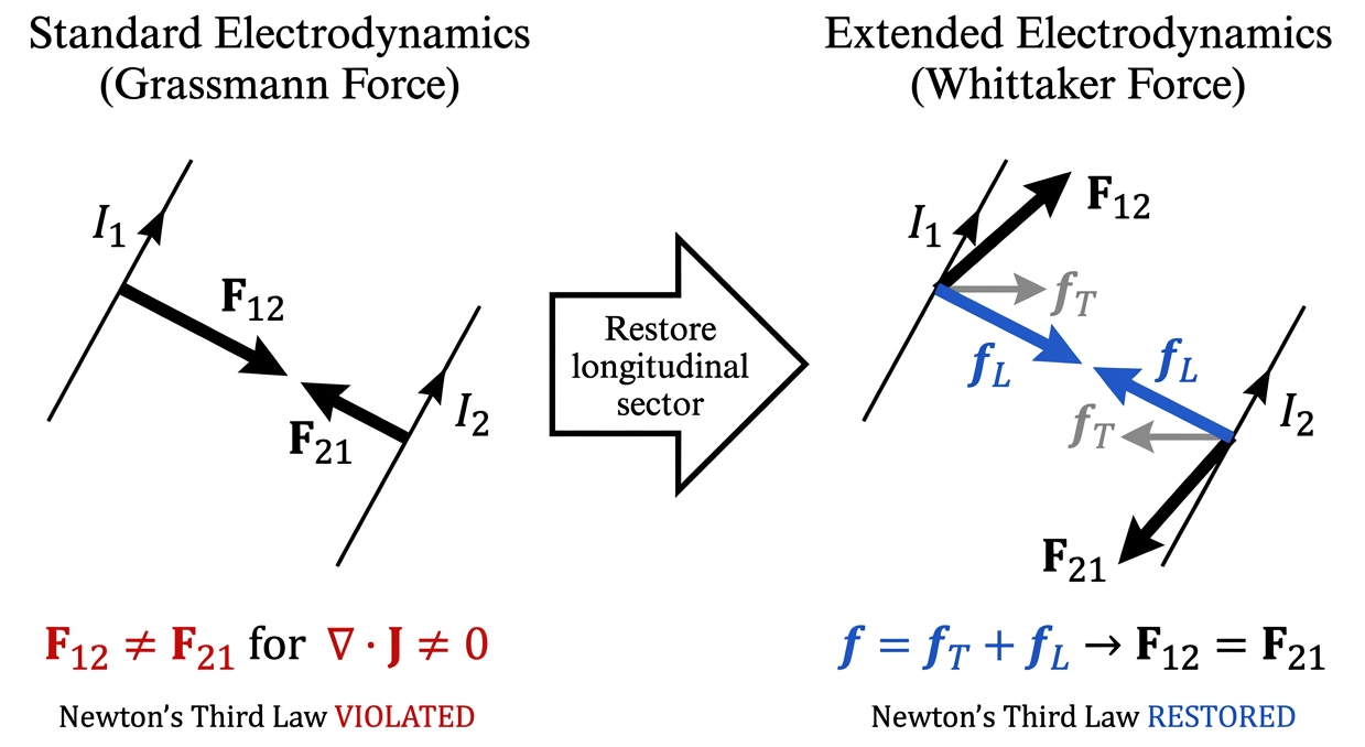
The deletion of the scalar-longitudinal sector has a consequence rarely discussed: standard electrodynamics violates Newton’s third law for non-closed current distributions. The Lorentz force between two current-carrying elements is not generally reciprocal for open circuits. Van Vlaenderen [34] showed that the Grassmann force law (the differential form underlying the Lorentz force) produces unbalanced forces whenever the current distribution has non-zero divergence — precisely the configurations where \(\nabla \cdot \mathbf{A} \neq 0\).
The resolution comes from the same scalar field that Extended Electrodynamics recovers. GCED [34] introduces a scalar magnetic field \(B_L\) mediating a longitudinal Ampere force \(\mathbf{f}_L\) alongside the standard transverse force \(\mathbf{f}_T\). The total Ampere force density \(\mathbf{f} = \mathbf{f}_L + \mathbf{f}_T\) satisfies Newton’s third law for both closed and open circuits. The reciprocal force law that emerges is Whittaker’s force law — a generalization of Grassmann’s that includes the longitudinal component the Lorenz gauge removes.
This is not an exotic prediction. It is testable in exploding-wire experiments, railgun physics, and any configuration involving non-divergence-free currents. The longitudinal forces have been observed experimentally but cannot be accounted for within standard Maxwell electrodynamics.
A fair objection: railgun anomalies and exploding-wire dynamics involve extreme conditions (high current densities, rapid phase transitions, magnetohydrodynamic instabilities) where attributing force discrepancies to a missing longitudinal component rather than to unmodeled material effects is not unique. However, the mathematical point is independent of any specific experiment: the Grassmann force law is provably non-reciprocal for \(\nabla \cdot \mathbf{J} \neq 0\), and Newton’s third law is a constraint that any complete theory must satisfy. Whether the longitudinal Ampere force is the correct resolution is an experimental question; that standard electrodynamics has a problem is a mathematical fact.
4.6 The Heaviside Energy Paradox
The deletion of degrees of freedom has consequences for energy accounting that are rarely acknowledged. The Poynting vector \(\mathbf{S} = \mathbf{E} \times \mathbf{B}/\mu_0\) is the standard measure of electromagnetic energy flow. But as Heaviside himself recognized, the Poynting vector is not unique: the curl of any vector field can be added to it without changing the total energy flux through any closed surface. The Poynting vector captures the divergent part of the energy flow; the curl addition — the Heaviside component — is divergence-free and therefore invisible to energy conservation arguments.
The Heaviside component is not small. Around a current-carrying conductor, the non-Poynting energy flow is enormously greater in magnitude than the Poynting component that enters the wire [2]. Almost all electromagnetic energy flowing near a conductor passes by without being intercepted. This is not a theoretical curiosity but a measurable fact: the energy density of the electromagnetic field around a wire vastly exceeds the energy delivered to the load.
Standard electrodynamics declares the Heaviside component unphysical because it does not contribute to net energy transfer across closed surfaces. But this declaration depends on the assumption that energy flow is fully characterized by \(\mathbf{E}\) and \(\mathbf{B}\). In the potential-primary formulation, energy flow has additional terms involving \(\mathbf{A}\) and \(\phi\) directly. Van Vlaenderen’s generalized Poynting vector [33] \(\mathbf{P} = \mathbf{E} \times \mathbf{B} - \mathbf{E}\,S\) provides a concrete mechanism: the scalar field \(S\) contributes an energy flux term \(-\mathbf{E}\,S\) that is longitudinal, carries its own energy density (\(\propto S^2\)), and operates even when \(\mathbf{B} = 0\). For scalar-longitudinal waves, the entire energy flux is carried by the \(-\mathbf{E}\,S\) channel, with the standard \(\mathbf{E} \times \mathbf{B}\) contribution vanishing identically. The Heaviside component may not be “excess” energy flowing nowhere — it may be energy flowing through the scalar channel that the field-primary Poynting vector structurally cannot represent.
4.7 The Potential Hierarchy
In 1903, Whittaker [41] proved that the general solution of the Laplace equation in three dimensions can be expressed as an integral over plane waves:
\[\phi(\mathbf{r}) = \int_0^{2\pi} f(x \cos\alpha + y \sin\alpha + iz,\;\alpha)\, d\alpha \tag{13}\label{eq:whittaker}\]
where \(f\) is an arbitrary function of two arguments. This means any static scalar potential — electrostatic or gravitational — is not a structureless quantity. It is an integral superposition of plane waves propagating in all directions.
A concrete example makes the point. The Coulomb potential \(\phi = q / (4\pi \varepsilon_0 r)\) satisfies the Laplace equation everywhere except the origin. Applying Whittaker’s theorem yields:
\[\frac{1}{r} = \frac{1}{2\pi}\int_0^{2\pi} \frac{1}{x\cos\alpha + y\sin\alpha + iz}\; d\alpha \tag{14}\label{eq:whittaker-coulomb}\]
The point charge’s apparently structureless \(1/r\) potential is revealed as a superposition of plane-wave-like functions over all azimuthal directions. Each term in the integrand depends on a single linear combination of coordinates — a directional mode that the gradient operation \(\mathbf{E} = -\nabla\phi\) cannot recover individually. The potential carries structural information that the field representation destroys upon differentiation. The equivalent Fourier-space representation makes this even more transparent:
\[\frac{1}{|\mathbf{r}|} = \frac{1}{2\pi^2} \int \frac{e^{i\mathbf{k}\cdot\mathbf{r}}}{k^2}\, d^3k \tag{15}\label{eq:fourier-coulomb}\]
Each Fourier mode \(e^{i\mathbf{k}\cdot\mathbf{r}}/k^2\) propagates in a definite direction \(\hat{\mathbf{k}}\). The potential is a sum over all such modes; the field is the gradient of this sum. Information about the individual mode structure is present in \(\phi\) but absent from \(\mathbf{E}\).
In the interpretation developed by later scalar wave theorists, the bidirectional structure of these wave pairs implies the simultaneous presence of time-forward and time-reversed components — though Whittaker’s original treatment is purely mathematical and does not make this physical claim. Indeed, Rodrigues and Trovon de Carvalho [28] identified specific mathematical limitations in Whittaker’s 1903 construction: the potential satisfies the Poisson equation (not Laplace, as Whittaker stated), the assumed emission spectrum is ad hoc, and the Fourier-decomposed fields are complex-valued rather than physically observable. These caveats do not invalidate the decomposition’s utility for the present argument — the structural point that potentials carry more information than fields survives intact — but they must be acknowledged to distinguish the rigorous mathematical content from overclaiming that has appeared in the subsequent literature.
Whittaker’s 1904 paper [42] extended this result to electrodynamics, showing that the complete electromagnetic field can be expressed through two scalar potential functions \(F\) and \(G\). The interference of these two scalar potentials generates all the field patterns of classical electrodynamics. Hillion [43] demonstrated that Whittaker’s two scalars are a special case of the more general Hertz potentials \((\Pi, \Omega)\), obtained by fixing an arbitrary unit vector to a specific direction (\(\mathbf{g} = \hat{\mathbf{z}}\)), with the identification \(F = \Pi\), \(G = -\Omega\). The Hertz potentials are direction-independent and more general; the four-potential is derived from them via \(\mathbf{A} = -\delta\Pi\) (with the Lorenz gauge emerging automatically from \(\delta^2 = 0\)), and the field tensor follows mechanically as \(F_{\mu\nu} = \partial_{[\mu}A_{\nu]}\). This establishes a potential hierarchy deeper than previously recognized:
Scalar wave equation (\(\partial^2\Phi = 0\)) \(\;\to\;\) Hertz potential \(\Pi\) \(\;\to\;\) Whittaker scalars \((F, G)\) \(\;\to\;\) Four-potential \((\phi, \mathbf{A})\) \(\;\to\;\) Fields \((\mathbf{E}, \mathbf{B})\)
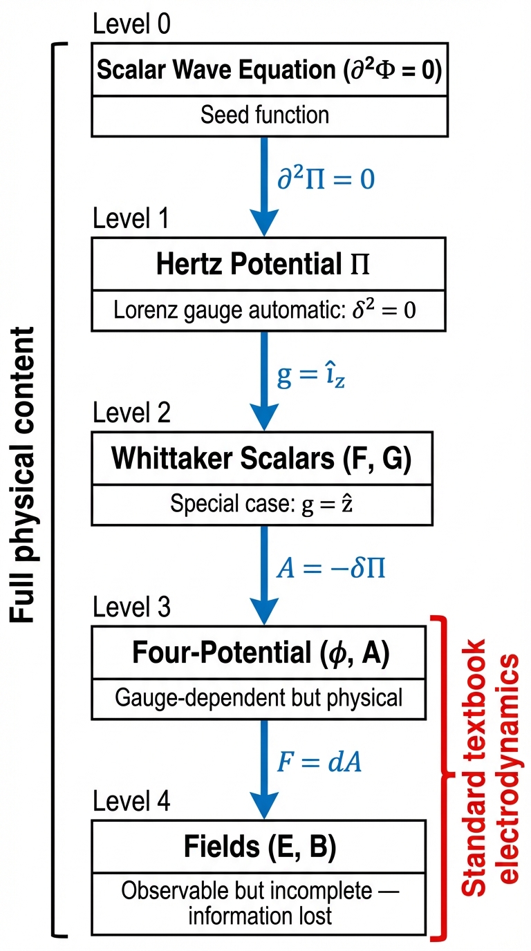
Each level of the potential hierarchy generates the next by a derivative operation. Each derivative operation is lossy — information present in the generating object is absent from the derived one. Standard electrodynamics operates at the bottom two levels. The Lorenz gauge, which at the four-potential level is an external constraint, is at the Hertz potential level an automatic identity (\(\delta^2 = 0\)). The gauge condition is not a physical law but an algebraic tautology of the deeper structure.
The connection to the scalar-longitudinal sector (Eq. (12)) is direct: Whittaker’s decomposition shows that potentials have internal wave structure; Extended Electrodynamics shows that relaxing the Lorenz gauge allows this structure to propagate as a dynamical field. The Whittaker decomposition provides the kinematic evidence for potential richness; EED provides the dynamical mechanism.
Mead [44] connected Whittaker’s scalar potentials to quantum mechanics through the superpotential \(\chi\), defined by \(\mathbf{A} = \nabla\chi\) and \(\phi = \partial\chi/\partial t\). In a superconductor, the macroscopic quantum phase \(\theta\) is directly proportional to the superpotential: \(\chi = (\hbar/q)\theta\). This connects the potential hierarchy to quantum coherence: the superpotential is (up to a constant) the quantum phase itself. The topological constraint that \(\theta\) must be single-valued modulo \(2\pi\) produces flux quantization (Eq. (9)) — showing that the potential hierarchy is not merely mathematical but determines the quantization conditions of macroscopic quantum systems.
A further degree of freedom invisible to the standard formulation has been identified in metamaterials research. Kaelberer et al. [45] demonstrated that electromagnetic fields in metamaterials require a toroidal dipole moment — a third multipole family beyond the electric and magnetic multipoles of the standard expansion. The associated order parameter, toroidization \(\mathbf{T}(t)\), is analogous to electric polarization \(\mathbf{P}\) and magnetization \(\mathbf{M}\): a macroscopic state variable that describes the material’s response to electromagnetic excitation. Standard electrodynamics has no mechanism to represent toroidization because it requires the interplay of longitudinal and transverse potentials — the same interplay that gauge fixing suppresses.
The standard formulation operates at the field level. It cannot see the scalar potential structure above — not because that structure is speculative, but because the Lorenz gauge and the ontological demotion made it invisible.
4.8 The Quantum Persistence of Deleted Modes
The deleted degrees of freedom are not merely a classical curiosity. They persist in quantum field theory. In Lorentz-gauge quantization, the four-potential \(A_\mu\) carries four polarization states per wave vector: two transverse, one longitudinal, and one scalar. The standard Gupta-Bleuler formalism handles the extra modes by introducing an indefinite-metric Hilbert space (with negative-norm “ghost” states) and filtering physical states via the subsidiary condition \(\partial_\mu A^{(+)\mu}|\psi\rangle = 0\). The longitudinal and scalar modes cancel pairwise in physical matrix elements but remain present in the operator algebra. Goto [46] demonstrated that this cancellation is not the only option: by allowing \(A_\mu\) to be non-Hermitian while preserving a Hermitian Hamiltonian, one obtains a positive-definite Hilbert space with no ghosts, no indefinite metric, and an \(S\)-matrix identical to Dyson’s standard formulation. In Goto’s construction, the longitudinal and scalar photon modes persist as independent dynamical variables. The Lorentz condition filters which states are physical — it does not delete the degrees of freedom from the theory’s dynamical structure.
The conventional identification of these modes as “unphysical” reflects a state-selection criterion, not a structural absence. The counterargument is that non-Hermitian operators may be mathematically admissible without being physically meaningful — a formal trick that preserves the \(S\)-matrix while inflating the ontology. But this objection cuts both ways: if the standard Gupta-Bleuler formalism introduces indefinite metrics and ghost states as mathematical artifacts of mode deletion, and Goto’s formalism avoids those artifacts at the cost of non-Hermiticity in unobservable fields, the question of which formalism is “merely formal” is not settled by appeal to convention. The “deleted” degrees of freedom were never absent from quantum electrodynamics. They were declared invisible.
The sharpest objection must be stated explicitly: in Gupta-Bleuler quantization, the scalar (timelike) photon mode has negative norm. This is a mathematical fact, not an artifact of a particular gauge choice. The standard theory handles this by restricting to a physical subspace where the negative-norm states decouple from all observables (the Ward identities guarantee this cancellation order by order in perturbation theory). If the scalar-longitudinal sector is promoted to physical status — as EED proposes classically and as Goto’s formalism permits quantum-mechanically — the question of whether negative-norm states contaminate the physical Hilbert space must be answered.
Three responses are available. First, Goto’s non-Hermitian construction produces a positive-definite Hilbert space with an \(S\)-matrix identical to the standard one; the negative norms are an artifact of insisting on Hermitian field operators, not a physical constraint. Second, EED as formulated by Reed and Hively is a classical framework. Its predictions — scalar-longitudinal wave propagation, Faraday cage penetration, modified Poynting vector — are classical observables that do not require quantization to test. Whether EED admits a consistent quantum extension is an open question, but the classical predictions stand independently of the answer. Third, the massive Stueckelberg theory (\(m > 0\)) is known to be renormalizable and unitary [36] — the compensating scalar ensures that all negative-norm states decouple exactly, as in the Standard Model’s electroweak sector. Whether the massless EED limit (\(m \to 0\), \(\gamma = 1\)) preserves this unitarity is the precise question that a future quantum treatment of EED must address.
This paper does not claim that the quantization problem is solved. It claims that the classical scalar-longitudinal sector is physically well-defined, experimentally testable, and invisible in the field-primary formulation — and that the quantum status of these modes is an open question that the standard formulation forecloses by convention rather than by proof.
4.9 The Time-Symmetric Sector
Wheeler and Feynman [12], [13] demonstrated that classical electrodynamics admits a fully time-symmetric formulation. Their central postulate replaces the standard retarded-only field with a time-symmetric combination: the electromagnetic field tensor acting on particle \(a\) due to particle \(b\) is
\[F^{\mu\nu}_{(b \to a)} = \frac{1}{2}\left(F^{\mu\nu}_{\mathrm{ret},b} + F^{\mu\nu}_{\mathrm{adv},b}\right) \tag{16}\label{eq:wf-field}\]
where \(F^{\mu\nu}_{\mathrm{ret},b}\) and \(F^{\mu\nu}_{\mathrm{adv},b}\) are the retarded and advanced Liénard-Wiechert fields of particle \(b\). This postulate follows from the Fokker action [12]:
\[S = -\sum_a m_a c \int ds_a - \sum_{a < b} e_a e_b \iint \delta\!\bigl[(x_a - x_b)^2\bigr]\, \dot{x}_a^\mu\, \dot{x}_{b\mu}\; ds_a\, ds_b \tag{17}\label{eq:fokker}\]
The delta function \(\delta[(x_a - x_b)^2]\) constrains interactions to the light cone and selects both retarded and advanced contributions with equal weight — this is the mathematical origin of the half-and-half structure. The theory eliminates self-interaction divergences entirely: there is no field of a particle acting on itself, only direct particle-particle action at a distance along the light cone.
Dirac had previously shown [47] that using half the difference between retarded and advanced fields eliminates the divergent self-energy of classical electron theory, avoiding the need for mass renormalization. The Wheeler-Feynman theory provides a physical mechanism for Dirac’s mathematical prescription: the absorber (the rest of the universe) responds with advanced waves that, when summed with each emitter’s time-symmetric field, produce the observed purely retarded radiation and the correct radiation reaction force.
The counterargument is substantive and must be examined honestly. The absorber theory requires the universe to be a “perfect absorber” — that all emitted radiation is eventually absorbed by the totality of matter in the universe. This is a cosmological boundary condition that is difficult to test independently. In an expanding universe with a cosmological horizon, radiation emitted beyond the horizon may never be absorbed, violating the perfect-absorber condition. Davies and Hogarth showed that the theory’s predictions depend on the cosmological model: in a matter-dominated Friedmann universe, the absorber condition is satisfied; in a radiation-dominated or de Sitter universe, it may fail. The theory therefore makes a testable cosmological prediction — but one that couples its electromagnetic content to the large-scale structure of the universe in a way that standard electrodynamics does not.
If the absorber condition fails, the Wheeler-Feynman formulation does not recover standard retarded radiation automatically. The time-symmetric field becomes an incomplete description, and additional boundary conditions must be imposed to select the retarded solution. The formulation degrades gracefully — it reduces to the standard theory with an explicit boundary condition rather than an implicit one — but it loses its explanatory advantage regarding the arrow of time.
The theory has not been extended to a fully satisfactory quantum version, though Cramer’s Transactional Interpretation of quantum mechanics [48] builds directly on the Wheeler-Feynman framework.
Despite these limitations, the mathematical point stands: the standard practice of discarding advanced solutions is not required by the equations. It is a boundary condition choice that eliminates physical content about the absorber structure of the universe. The time-symmetric sector is what Act 2 deleted when it privileged retarded solutions.
Cramer [48] extended the Wheeler-Feynman framework into quantum mechanics with the Transactional Interpretation: quantum events are “handshakes” between retarded offer waves (\(\psi\)) and advanced confirmation waves (\(\psi^*\)). The critical observation is that \(\psi^*\) — the complex conjugate of the wave function — is an advanced wave. Wigner’s time-reversal operator in quantum mechanics is complex conjugation. The Born rule \(P = |\psi|^2 = \psi\psi^*\) already contains both time directions: the retarded wave \(\psi\) propagating forward and the advanced wave \(\psi^*\) propagating backward. Standard quantum mechanics uses both components in every probability calculation but does not acknowledge the time-reversed component as physically meaningful.
This means the “deleted” time-symmetric sector was never truly deleted from quantum mechanics. It was hidden in the formalism’s use of \(\psi^*\) — present in every overlap integral, every matrix element, every expectation value. The deletion occurred at the interpretive level: the physics kept the mathematics of advanced waves while the narrative declared them unphysical. The time-symmetric sector is hiding in plain sight in the complex conjugate structure of quantum mechanics.
4.10 The Electromagnetic-Gravitational Bridge
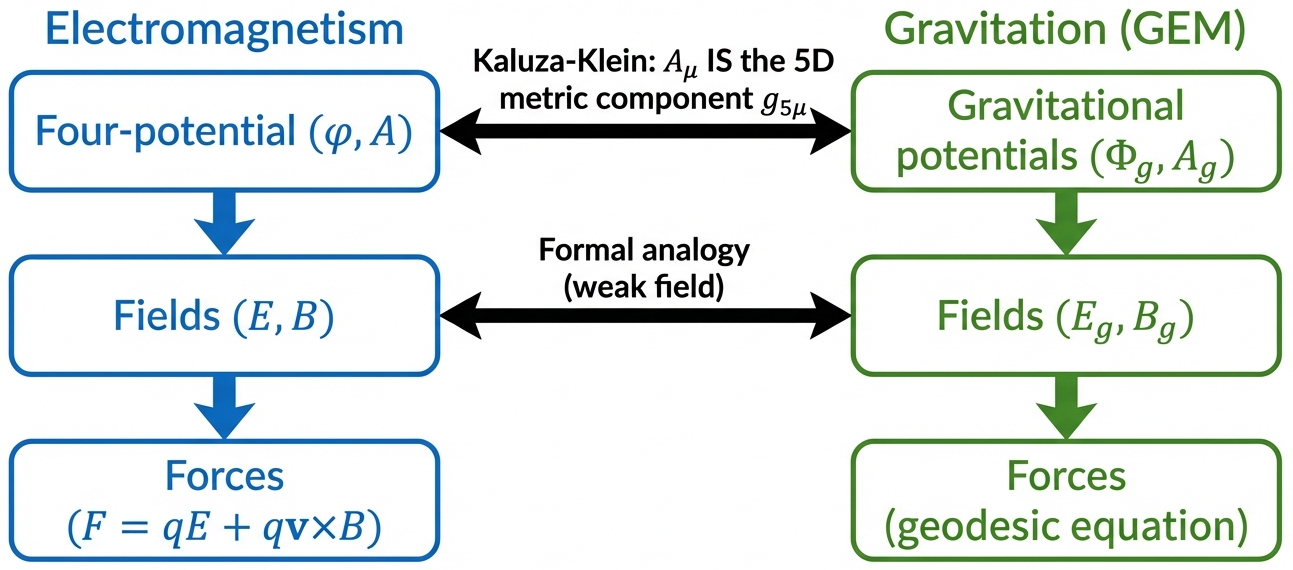
In the weak-field limit of general relativity, the Einstein field equations reduce to a set of equations formally analogous to Maxwell’s equations — gravitoelectromagnetism (GEM) [49]. The analogy introduces a gravitoelectric field \(\mathbf{E}_g\) and a gravitomagnetic field \(\mathbf{B}_g\), derived from a gravitational scalar potential \(\Phi_g\) and vector potential \(\mathbf{A}_g\):
\[\mathbf{E}_g = -\nabla \Phi_g - \frac{1}{2c}\frac{\partial \mathbf{A}_g}{\partial t}, \quad \mathbf{B}_g = \nabla \times \mathbf{A}_g \tag{18}\label{eq:gem-potentials}\]
These fields satisfy four equations structurally identical to Maxwell’s equations [49]:
\begin{align} \nabla \cdot \mathbf{E}_g &= -4\pi G \rho \tag{19}\label{eq:gem-gauss} \\ \nabla \cdot \mathbf{B}_g &= 0 \tag{20}\label{eq:gem-divb} \\ \nabla \times \mathbf{E}_g &= -\frac{1}{c}\frac{\partial \mathbf{B}_g}{\partial t} \tag{21}\label{eq:gem-faraday} \\ \nabla \times \mathbf{B}_g &= -\frac{4\pi G}{c}\,\mathbf{J}_g + \frac{1}{c}\frac{\partial \mathbf{E}_g}{\partial t} \tag{22}\label{eq:gem-ampere}\end{align}
where \(\rho\) is mass density, \(\mathbf{J}_g = \rho\mathbf{v}\) is mass current density, and the negative signs (relative to electromagnetism) reflect that gravity is attractive. The factor of \(1/2\) in Eq. (18) has no electromagnetic counterpart. It originates in the linearized Einstein equations: writing the metric as \(g_{\mu\nu} = \eta_{\mu\nu} + h_{\mu\nu}\), the off-diagonal components \(h_{0i}\) enter the geodesic equation with a coefficient of \(2\) relative to the Newtonian potential \(h_{00}\), producing \(\mathbf{A}_g = -c^2 (h_{01}, h_{02}, h_{03})/2\). The \(1/2\) thus reflects the spin-2 tensor structure of gravity [49] — a fundamental difference that prevents the analogy from being exact at all orders. This analogy is experimentally confirmed. The Gravity Probe B mission [50] measured frame-dragging — the gravitomagnetic effect — around Earth at \(37.2 \pm 7.2\) milliarcseconds per year, in agreement with the GEM prediction. Moving mass generates a gravitational analogue of the magnetic vector potential, and the gravitomagnetic field \(\mathbf{B}_g\) produces measurable effects on orbiting gyroscopes.
Li and Torr [51] demonstrated that the London equations can be extended to incorporate gravitomagnetic fields. In a superconductor, the Cooper pair condensate physically fixes \(\mathbf{A}\) (London gauge). Li and Torr showed that the same condensate may simultaneously fix the gravitational vector potential \(\mathbf{A}_g\) through a gravitomagnetic London moment:
\[\mathbf{B}_g = -\frac{2m}{e}\,\boldsymbol{\omega} \tag{23}\label{eq:grav-london}\]
where \(\boldsymbol{\omega}\) is the angular velocity of the superconductor. This prediction connects the electromagnetic London equation (Eq. (8)) to gravitomagnetic effects through the mass-to-charge ratio of the Cooper pair — the same ratio that determines the flux quantum \(h/2e\). If the superconductor physically enforces potential primacy for \(\mathbf{A}\) (as the London equation establishes), and if the same mechanism extends to \(\mathbf{A}_g\) (as Li and Torr predict), then superconductors provide a direct experimental bridge between electromagnetic and gravitational potential primacy — not an analogy but a physical coupling mediated by the same condensate.
In the potential-primary interpretation, the EM-gravity analogy gains additional depth. If both electromagnetic and gravitational phenomena are fundamentally described by connections (potentials) rather than curvatures (fields), then the shared geometric structure suggests a deeper relationship than the formal analogy alone. NASA’s Breakthrough Propulsion Physics program [40] explored whether specially conditioned electromagnetic configurations — designed to maximize vector potential disturbances — could produce measurable gravitational effects. The program documented that toroidal geometries generate \(\mathbf{A}\)-field patterns extending far beyond the device boundary, where \(\mathbf{E}\) and \(\mathbf{B}\) vanish. No positive gravitational results were reported.
The connection between electrodynamics and gravitation deepens considerably in the Kaluza-Klein framework [52], [53]. By extending spacetime from four to five dimensions, Kaluza showed that the electromagnetic four-potential \(A_\mu\) appears as the off-diagonal components of the five-dimensional metric tensor \(g_{5\mu}\). In this formulation, gauge transformations are coordinate transformations in the fifth dimension, and electric charge is momentum in the fifth dimension. The vector potential is not analogous to the gravitational metric — it is part of the gravitational metric in five dimensions. Deleting degrees of freedom from \(A_\mu\) therefore deletes components of the higher-dimensional gravitational field.
The superpotential formulation makes this connection precise through a striking identification: the gravitational potential \(\Phi_g\) is related to the divergence of \(\mathbf{A}\) — precisely the term that the Lorenz gauge eliminates. If \(\nabla \cdot \mathbf{A}\) carries gravitational information, then gauge-fixing the electromagnetic potentials simultaneously hides gravitational degrees of freedom. This is not an analogy. It is a mathematical consequence of the Kaluza-Klein embedding: gauge freedom in four dimensions is geometric freedom in five dimensions, and constraining one constrains the other.
A more speculative connection deserves mention with appropriate caveats. Woodward [54], extending Sciama’s formulation of Mach’s principle [55], predicted that time-varying energy content in a system produces transient fluctuations in its inertial mass, mediated by the scalar gravitational potential \(\Phi_g\):
\[\delta m(t) \propto \frac{1}{\Phi_g}\frac{\partial^2 E}{\partial t^2} - \frac{1}{\Phi_g^2}\left(\frac{\partial E}{\partial t}\right)^2 \tag{24}\label{eq:woodward}\]
The Woodward effect is explicitly about the scalar potential as a physical mediator of inertial effects. NASA has funded experimental programs testing this prediction [40], with reported thrust measurements from capacitors undergoing rapid energy changes. However, the experimental status is contested: thrust measurements at the micro-Newton level are susceptible to systematic errors (thermal expansion, electromagnetic interference, center-of-mass shifts), and no independent replication has confirmed the effect. The theoretical derivation itself depends on Sciama’s formulation of Mach’s principle, which is one of several competing implementations and not uniquely determined by general relativity. This prediction is included because it illustrates how potential primacy connects to the origin of inertia — not because the effect is established. The reader should treat Eq. (24) as a theoretical possibility, not as an observational result on the same footing as the Aharonov-Bohm phase or flux quantization.
The limits of this analogy deserve equal emphasis: GEM is a weak-field, slow-motion approximation. Full general relativity is a theory of spacetime curvature, not of gravitational potentials, and it has no simple potential-primary reformulation. The GEM analogy breaks down for strong fields, relativistic velocities, and nonlinear gravitational effects. The spin-2 nature of gravity (reflected in the factor of \(1/2\) above and the tensorial source) means the analogy is structural, not fundamental — the graviton, if it exists, has different quantum numbers than the photon. Whether potential primacy in electrodynamics implies potential primacy in gravitation remains an open question. What the GEM formalism does establish is that if the analogy holds at the potential level, then the same vector potential configurations that produce electromagnetic effects in field-free regions (Aharonov-Bohm) may probe gravitational degrees of freedom.
4.11 The Vacuum Coupling
The quantum vacuum is structured. Quantum electrodynamics predicts fluctuating electromagnetic fields even in the ground state, producing measurable effects: the Casimir force between conducting plates, the Lamb shift in hydrogen, spontaneous emission from excited atoms. These are not speculative predictions — they are confirmed to high precision.
In the field-primary formulation, coupling to the vacuum requires engineering field configurations (boundary conditions on \(\mathbf{E}\) and \(\mathbf{B}\)) that modify the mode structure of vacuum fluctuations. The Casimir effect is the canonical example: two conducting plates exclude long-wavelength modes between them, creating a net force.
In the potential-primary formulation, a more direct coupling channel opens. The vector potential \(\mathbf{A}\) polarizes the quantum vacuum and influences quantum phase even in regions where \(\mathbf{E} = 0\) and \(\mathbf{B} = 0\) — this is the Aharonov-Bohm effect applied to vacuum fluctuations. Wilson et al. [56] demonstrated the dynamical Casimir effect using a SQUID-based circuit: by rapidly modulating the effective boundary condition (the inductance of the SQUID, which is controlled by the magnetic flux \(\Phi = \oint \mathbf{A} \cdot d\mathbf{l}\)), they created real photon pairs from the vacuum. The boundary was not a moving mirror but a modulated potential — a direct demonstration that potential configurations, not just field configurations, couple to vacuum structure.
Graham and Lahoz [57] provided earlier evidence of vacuum coupling by measuring static electromagnetic angular momentum in vacuum — demonstrating that the crossed-field configuration \(\mathbf{E} \times \mathbf{B}\) carries real momentum even in empty space. The vacuum acts as a reservoir of angular momentum, consistent with Lorentz’s hypothesis of an inertial medium.
Haisch, Rueda, and Puthoff [58] proposed that inertial mass itself is not intrinsic but emergent: an electromagnetic drag force from the zero-point field (ZPF) acting on accelerated charges. Building on Sakharov’s 1968 proposal [59] that gravity is induced by vacuum fluctuations, the Haisch-Rueda-Puthoff (HRP) model identifies inertia as the resistance of the ZPF to acceleration. The ZPF appears isotropic to uniformly moving charges but asymmetric to accelerated charges, producing a back-reaction force proportional to acceleration — \(f = ma\) as an emergent relation rather than a fundamental law. If this model is correct, then the deleted degrees of freedom include the mechanism by which matter acquires mass: the coupling between the vector potential and the structured vacuum. This model has not achieved consensus. The calculation requires specific assumptions about the ZPF spectrum and the nature of the charge-vacuum interaction that remain debated. But the conceptual point survives independent of the specific model: the potential-primary formulation opens coupling channels to the vacuum that the field-primary formulation cannot represent, because \(\mathbf{A}\) extends into regions where \(\mathbf{E}\) and \(\mathbf{B}\) do not.
5 Engineering Implications
If the deleted content is restored, what engineering possibilities emerge? Each deleted sector identified in Section 4 opens a specific engineering design space that the field-primary formulation cannot represent.
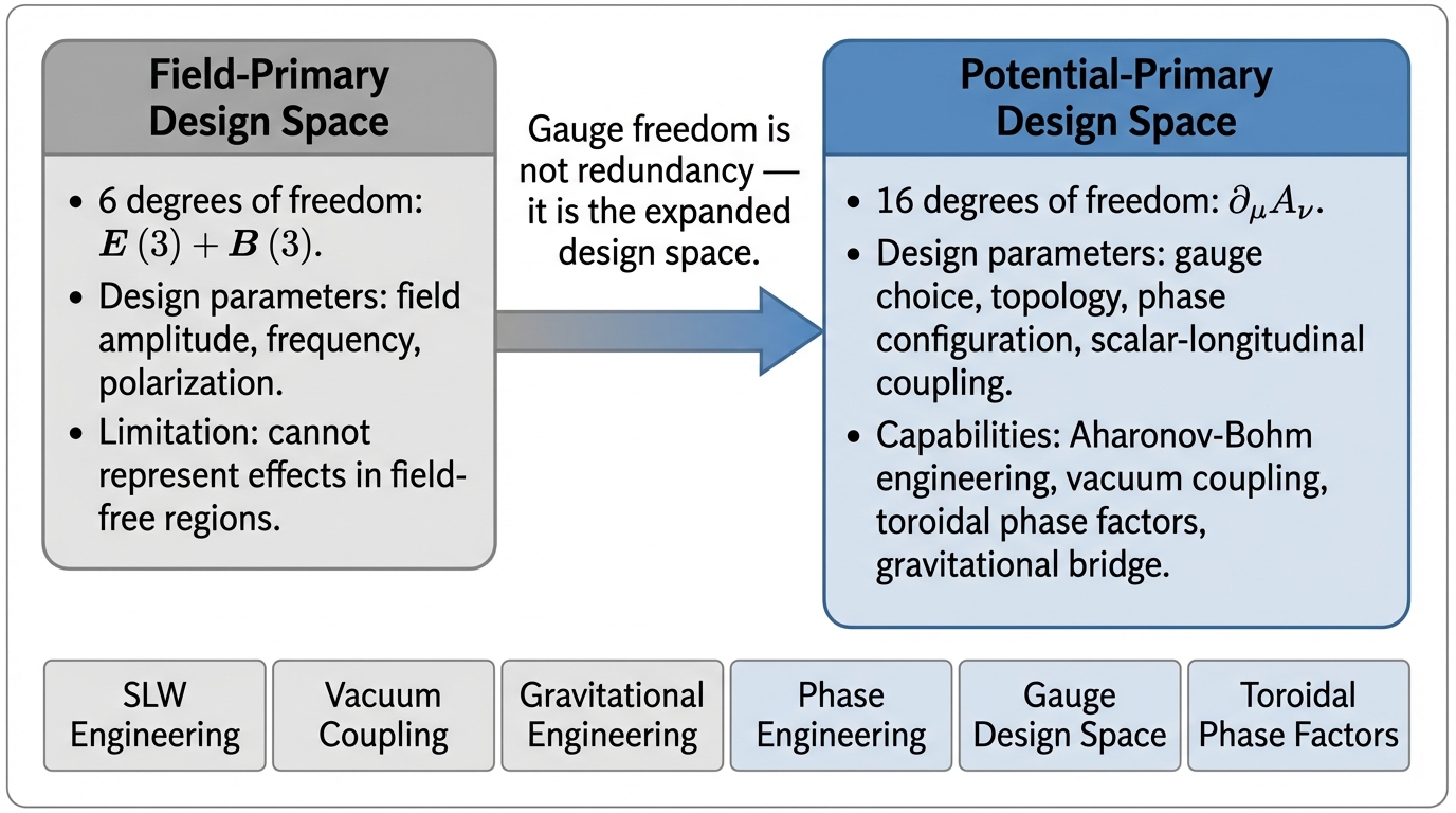
5.1 Scalar-Longitudinal Wave Engineering
If confirmed by independent replication, the EED predictions (Section 4.4) — skin-effect immunity, Faraday-cage penetration, \(1/r^2\) attenuation, monopolar reception — would translate directly into engineering applications for communication, sensing, and energy transfer through conductive barriers. The dispersion relation for SLW in curved spacetime connects to the Hubble constant and the Ricci tensor [4], suggesting that the scalar-longitudinal sector bridges electrodynamics and gravitation at the wave-propagation level.
5.2 Vacuum Coupling via Potential Configurations
The dynamical Casimir effect (Section 4.11) demonstrates that potential modulation creates real particles from the vacuum. Toroidal current configurations generate \(\mathbf{A}\)-field patterns extending far beyond the device boundary, where \(\mathbf{E}\) and \(\mathbf{B}\) vanish [40]. At resonant frequencies determined by the geometry, the vector potential disturbance is maximized through constructive interference. This suggests that systems which are electrically closed could in principle be open in terms of potential coupling — an engineering possibility that the field-primary formulation cannot even formulate.
5.3 Gravitational Engineering at the Potential Level
If potential primacy extends to gravitation (Section 4.10), electromagnetic configurations — particularly toroidal geometries that generate strong \(\mathbf{A}\)-fields in field-free regions — may probe gravitational degrees of freedom through the shared connection geometry. This remains a theoretical possibility, not a demonstrated effect.
5.4 Phase Engineering
SQUIDs already exploit flux quantization (Eq. (9)) — the macroscopic consequence of phase engineering via \(\mathbf{A}\). Berry’s geometric phase [23] generalizes the principle: engineering the connection (the potential configuration) engineers the phase evolution of quantum systems traversing that configuration. The question is not whether phase engineering works — it does — but what further applications become visible when the full potential hierarchy, including the superpotential structure (Section 4.7), is available as a design space.
5.5 Gauge Freedom as Design Space
The standard narrative treats gauge freedom as mathematical redundancy. The potential-primary perspective inverts this: gauge freedom is an unexploited engineering parameter space. Within the space of all potential configurations that produce the same fields, different configurations produce different non-field effects: different Aharonov-Bohm phases, different vacuum polarization patterns, different topological structures.
The analogy to canonical versus kinetic momentum makes this concrete. In the presence of an electromagnetic field, the canonical momentum \(\mathbf{p}_{\text{can}} = m\mathbf{v} + q\mathbf{A}\) is gauge-dependent, while the kinetic momentum \(\mathbf{p}_{\text{kin}} = m\mathbf{v}\) is gauge-invariant. Standard physics uses kinetic momentum and discards the gauge-dependent part. But the canonical momentum is what the Hamiltonian uses, what determines quantum phase evolution, and what superconductors physically enforce. The “gauge-dependent” part carries the engineering content.
5.6 Toroidal Phase Factor Engineering
The topological structure of toroidal geometries (Section 4.1) is essential: the torus is the simplest multiply connected geometry that produces field-free regions with non-zero \(\mathbf{A}\). Its topology can promote the gauge group from \(U(1)\) to \(SU(2)\) under specific excitation conditions [14], enabling non-Abelian phase factors that have no representation in terms of fields alone. Engineering the topology of the potential configuration — not just the amplitude of the fields — is the distinctive capability that the potential-primary formulation offers.
6 Discussion
The argument of this paper is structural, not speculative. Three historical simplifications deleted physical content from electrodynamics. The deleted content can be precisely identified. When it is restored — through gauge-free formulations, superpotential decompositions, time-symmetric theories, and the gravitational analogy — engineering possibilities emerge that the standard formulation structurally hides.
What this paper adds is the synthesis: the Aharonov-Bohm effect, Berry phase, Extended Electrodynamics, Whittaker’s decomposition, the Wheeler-Feynman absorber theory, and the GEM analogy are not isolated results in separate subfields. They are windows onto the same reality — a potential-primary electrodynamics richer than the one textbooks teach. The standard formulation is not wrong. It is incomplete in ways that have engineering consequences.
The standard objection — that gauge freedom makes potentials unphysical — fails on examination. Gauge freedom constrains the representation of \(\mathbf{A}\), not its physical content. The gauge-invariant quantities (enclosed flux, holonomy, geometric phase) are precisely the quantities that make the Aharonov-Bohm effect, superconductor physics, and Berry phase possible. As Feynman concluded: “In our sense then, the \(A\)-field is ‘real.’ ” [24]
6.1 Why Does Modern Physics Work Without Potential Primacy?
The obvious objection is this: if potential primacy is physically important, why does the entire edifice of modern physics — QED, the Standard Model, every precision measurement — work perfectly well in the field-primary formulation? Why should anyone care about degrees of freedom that 150 years of physics successfully ignored?
The answer has three parts.
First, modern physics does use potential primacy — it simply does not call it that. The Standard Model is a gauge theory. Its fundamental variables are connections (gauge potentials), not curvatures (field strengths). The photon field \(A_\mu\) is the \(U(1)\) connection; the gluon fields are the \(SU(3)\) connection; the \(W\) and \(Z\) are the \(SU(2) \times U(1)\) connection. Every Feynman diagram is computed from propagators of these potentials, not from propagators of \(\mathbf{E}\) and \(\mathbf{B}\). The Standard Model already implements potential primacy at the quantum level. The disconnect is not between the physics and potential primacy — it is between the physics and the textbook narrative that accompanies it.
The persistence of these modes in canonical QFT is examined in Section 4.8. The same preference operates in engineering: finite element solvers for computational electromagnetics have used the vector potential \(\mathbf{A}\) as their primary variable for decades [60]. The curl-curl equation for \(\mathbf{A}\) automatically enforces \(\nabla \cdot \mathbf{B} = 0\), and \(\mathbf{A}\)’s tangential continuity across material interfaces simplifies discretization where \(\mathbf{E}\) and \(\mathbf{B}\) are discontinuous. For superconductor modeling, \(\mathbf{A}\) is the only viable primary variable, since the London constitutive relation (Eq. (8)) defines the supercurrent as a direct function of \(\mathbf{A}\) itself. Industry-standard tools solve for potentials; textbooks teach fields. The disconnect is pedagogical, not physical.
Second, the field-primary formulation succeeds because the phenomena it was designed to describe are transverse. Electromagnetic radiation, scattering, and the precision tests of QED all involve transverse photon exchange. The transverse sector of electrodynamics is identical in the field-primary and potential-primary formulations — they diverge only in the longitudinal and scalar sectors that standard experiments do not probe. The success of QED is real but does not speak to the completeness of the theory with respect to non-transverse degrees of freedom.
Third, gauge freedom is a feature of the description, not of nature. The argument that potentials are unphysical because they are gauge-dependent proves only that any single gauge-fixed representation of \(\mathbf{A}\) underdetermines the physical content. The gauge-invariant quantities — enclosed flux, holonomy, geometric phase, Wilson loops — are precisely the quantities that make the Aharonov-Bohm effect, superconductor physics, and Berry phase possible. These quantities are defined in terms of potentials, not fields. Gauge freedom constrains the representation of \(\mathbf{A}\), not its ontological status — which is an argument for its richness, not its unreality.
The field-primary formulation is not wrong. It is a consistent restriction to the transverse sector of a richer theory. The question this paper raises is not whether the restriction works — it does — but whether the restricted theory can see the full engineering design space. The answer, given the evidence in Section 4, is that it cannot.
6.2 Gauge Fixing as Information Loss
The argument of this paper can be stated in information-theoretic terms. The four-gradient \(\partial_\mu A_\nu\) contains 16 kinematic components. The electromagnetic field tensor \(F_{\mu\nu}\) retains 6. The projection from 16 to 6 is a lossy compression — and unlike data compression, there is no decoder that recovers the original from the compressed version. The fields do not determine the potentials uniquely; that is precisely what gauge freedom means. The kinematic content of \(S_{\mu\nu}\) is irreversibly lost when physics works exclusively with \(F_{\mu\nu}\).
This compression discards more than redundant labeling. The symmetric part \(S_{\mu\nu}\) transforms under gauge as \(S_{\mu\nu} \to S_{\mu\nu} + \partial_\mu\partial_\nu\chi\), so it is gauge-dependent. But gauge dependence does not imply physical emptiness. The four-potential \(A_\mu\) is equally gauge-dependent, yet it carries physical content that the gauge-invariant \(F_{\mu\nu}\) cannot reconstruct: holonomy (the Aharonov-Bohm phase), flux quantization (the London constraint), and the canonical momentum that superconductors physically enforce. The principle is general: gauge-dependent fields can encode gauge-invariant physics through the observables constructed from them.
The same principle applies to \(S_{\mu\nu}\). Its trace \(\partial_\mu A^\mu\) is gauge-dependent in the standard theory (it transforms as \(\partial_\mu A^\mu \to \partial_\mu A^\mu + \Box\chi\)). But in Extended Electrodynamics (\(\gamma = 1\) in the Stueckelberg Lagrangian), the gauge freedom is eliminated by construction: the gauge-fixing term that standard electrodynamics imposes as a constraint is promoted to a dynamical term in the Lagrangian. The resulting theory has no residual gauge symmetry, and the scalar field \(C = \partial_\mu A^\mu\) acquires its own wave equation, energy density, and source coupling. These dynamical properties are not gauge-dependent — they are properties of a gauge-free theory.
A common objection deserves explicit address. In the standard Stueckelberg mechanism for massive electrodynamics (\(m > 0\)), the compensating scalar field is introduced precisely to restore gauge invariance, and it can be gauged away (unitary gauge reduces Stueckelberg to Proca). This makes the standard Stueckelberg scalar “pure gauge.” But in EED (\(\gamma = 1\), \(m = 0\)), the situation is structurally different: the scalar field \(C\) is not a compensator introduced to absorb gauge variation — it is the Lorenz divergence itself, promoted from a constraint (\(C = 0\)) to a dynamical variable (\(\Box C = \text{sources}\)). The distinction is between a field that exists to be gauged away and a field that exists because the gauge was removed. Whether this distinction survives quantization — in particular, whether the resulting quantum theory is unitary and ghost-free — is addressed in Section 4.8.
In the language of information theory, gauge fixing is an irreversible operation: it maps a larger state space onto a smaller one with no inverse. The information lost includes holonomy, scalar-longitudinal coupling, and topological structure that the field representation cannot reconstruct. The Aharonov-Bohm effect is the physical proof that the compression is lossy: there exist physically distinguishable states that map to the same field configuration but different potential configurations.
6.3 Implications for Quantum Mechanics
The connection between deleted degrees of freedom and quantum mechanics runs deeper than the Aharonov-Bohm effect. Three observations converge:
Cramer’s identification of \(\psi^*\) as an advanced wave implies that quantum mechanics already incorporates the time-symmetric sector that Act 2 deleted from classical electrodynamics. The Born rule \(P = \psi\psi^*\) is a product of retarded and advanced waves. The “measurement problem” may be, in part, a consequence of interpreting as paradoxical a mathematical structure that the Wheeler-Feynman framework renders natural.
Mead’s identification [44] of the superpotential \(\chi\) with the quantum phase \(\theta\) (via \(\chi = \hbar\theta/q\)) implies that quantum phase evolution is motion in the potential hierarchy. Gauge transformations \(\mathbf{A} \to \mathbf{A} + \nabla\chi\) are shifts in the superpotential, which are shifts in the quantum phase. The “unphysical” gauge freedom of classical electrodynamics is the physical phase freedom of quantum mechanics.
Taylor relaxation [27] demonstrates that discrete states can emerge from topological conservation laws without quantization in the quantum-mechanical sense. Turbulent plasmas relax into states labeled by winding numbers — integers that arise from the topology of the magnetic helicity, not from \(\hbar\). If “classical quantization from topology” is possible in plasma physics, the boundary between classical and quantum may be less fundamental than conventionally assumed — and the deleted topological degrees of freedom (Section 4.1) may be relevant to the foundations of quantum mechanics itself.
6.4 Limitations and Open Questions
This paper does not claim that restoring deleted degrees of freedom immediately yields practical devices. The engineering categories in Section 5 require theoretical development, experimental verification, and substantial engineering effort. Several specific limitations deserve acknowledgment:
Preliminary experimental results for scalar-longitudinal waves [38] are consistent with EED predictions but have not been independently replicated. Until they are, EED remains a mathematically consistent extension with suggestive but not conclusive experimental support.
The Whittaker decomposition’s physical interpretation (particularly the time-reversal reading of phase-conjugate wave pairs) goes beyond Whittaker’s original mathematical result. The decomposition is proven; the ontological interpretation is not.
The gravitational extension via the GEM analogy is a formal analogy in the weak-field limit. Whether potential primacy extends to full general relativity — and whether electromagnetic configurations can produce measurable gravitational effects — remains an open experimental question with no positive results to date.
The Wheeler-Feynman absorber theory, while mathematically consistent, requires specific assumptions about cosmological boundary conditions that are difficult to test independently.
The Haisch-Rueda-Puthoff model of inertia as ZPF drag, while published in Physical Review A, has not achieved consensus. The specific form of the charge-vacuum interaction and the ZPF spectrum assumptions remain debated.
The Kaluza-Klein framework, while mathematically elegant, requires a fifth dimension whose physical status is unclear. Compactification to unobservable scales is assumed but not derived.
Woodward’s Mach effect thruster results, while NASA-funded, remain contested. Systematic errors in thrust measurement at the micro-Newton level are difficult to exclude definitively.
The quantization of EED remains an open problem. The massive Stueckelberg theory is known to be renormalizable and unitary, but whether the massless EED limit (\(m \to 0\), \(\gamma = 1\)) preserves these properties — in particular, whether the scalar-longitudinal sector is ghost-free at the quantum level — has not been demonstrated. The classical predictions of EED (scalar-longitudinal wave propagation, modified energy flow) are independent of this question, but a complete theoretical foundation requires it to be answered.
A necessary distinction: the arguments in this paper must not be confused with the “O(3) electrodynamics” of Evans and the AIAS group, which operates in superficially similar thematic territory (extended Maxwell equations, scalar waves, potential ontology). Trovon de Carvalho and Rodrigues [28] have demonstrated that the AIAS program rests on elementary group-theoretic errors (confusing \(U(1)\) with \(O(2)\), inverting the covering-group relation between \(SU(2)\) and \(SO(3)\)), a fictitious \(B^{(3)}\) field refuted by experiment, and fundamental misunderstandings of gauge theory. The Evans program is mathematically incoherent. The extended electrodynamics discussed here (Section 4.3) derives from the Stueckelberg Lagrangian, is supported by Woodside’s uniqueness theorems, and has been arrived at independently by multiple research groups over two decades. The two programs share terminology; they share nothing else.
What this paper does claim is that these engineering categories are invisible in the field-primary formulation — not because they are speculative, but because the formulation structurally cannot represent them. Restoring the full theory does not guarantee applications. It makes them conceivable.
7 Conclusion
Every time physics chose mathematical convenience over physical completeness, it deleted an engineering degree of freedom. Heaviside deleted the scalar-longitudinal sector and the scalar part of the quaternion product. The Lorenz gauge deleted the independent content of \(\nabla \cdot \mathbf{A}\), the seventh field component \(T\), and advanced solutions. The ontological demotion deleted the motivation to investigate what had been removed. Together, they reduced a 16-component theory to a 6-component one and declared the missing 10 components unphysical.
The Aharonov-Bohm effect proved the demotion was wrong. The Maxwell-Lodge effect proved it classically. The fiber bundle formulation proved it was topologically destructive. Extended Electrodynamics — derived independently by Van Vlaenderen [33], Hively and Giakos [35], and Reed and Hively [4] — showed what the Lorenz gauge hides. The Vector Potential Transformer showed it is real enough to build patented devices on. Newton’s third law showed that standard electrodynamics fails for open circuits — and that restoring the longitudinal force restores the symmetry. Whittaker and Hertz [43] showed the potential hierarchy extends above the four-potential. Goto [46] showed that even in canonical QFT, the “deleted” modes persist as independent dynamical variables. Wheeler-Feynman showed that time symmetry is physically consistent — and Cramer showed it was hiding in quantum mechanics all along. Gravity Probe B showed that potential primacy extends to gravitation. Kaluza-Klein showed it was gravitation. The dynamical Casimir effect showed that potential modulation creates real particles from the vacuum.
The physics that textbooks skip is not exotic. It is the physics that Heaviside found inconvenient, that the Lorenz gauge made invisible, and that a century of ontological prejudice kept hidden. The full potential tensor \(\partial_\mu A_\nu\) — all 16 components — contains scalar-longitudinal propagation, topological structure, vacuum coupling channels, gravitational degrees of freedom, and a time-symmetric sector that quantum mechanics already uses without acknowledging. Restoring it is not a revolution. It is a correction — and the engineering consequences of that correction, beginning with the non-Hermitian topology of exceptional point systems and the experimental search for scalar-longitudinal wave signatures, are the subject of the work that follows.
References
[1] N. Osakabe et al., “Experimental confirmation of Aharonov-Bohm effect using a toroidal magnetic field confined by a superconductor,” Physical Review A, vol. 34, no. 2, pp. 815–822, 1986, doi: 10.1103/PhysRevA.34.815.
[2] O. Heaviside, Electromagnetic theory, vol. 1. London: The Electrician Printing; Publishing Company, 1893.
[3] J. C. Maxwell, A treatise on electricity and magnetism, vols. 1 – 2. Oxford: Clarendon Press, 1873.
[4] D. Reed and L. M. Hively, “Implications of gauge-free extended electrodynamics,” Symmetry, vol. 12, no. 12, p. 2110, 2020, doi: 10.3390/sym12122110.
[5] H. von Helmholtz, “Über die Erhaltung der Kraft.” 1847.
[6] D. Hestenes, Space-time algebra, 2nd ed. Birkhäuser, 2015. doi: 10.1007/978-3-319-18413-5.
[7] C. Doran and A. Lasenby, Geometric algebra for physicists. Cambridge University Press, 2003. doi: 10.1017/CBO9780511807497.
[8] J. D. Jackson and L. B. Okun, “Historical roots of gauge invariance,” Reviews of Modern Physics, vol. 73, no. 3, pp. 663–680, 2001, doi: 10.1103/RevModPhys.73.663.
[9] J. W. Gibbs and E. B. Wilson, Vector analysis. New York: Charles Scribner’s Sons, 1901.
[10] O. D. Jefimenko, Electromagnetic retardation and theory of relativity, 2nd ed. Star City, WV: Electret Scientific Company, 2004.
[11] L. V. Lorenz, “On the Identity of the Vibrations of Light with Electrical Currents,” Philosophical Magazine, vol. 34, no. 230, pp. 287–301, 1867.
[12] J. A. Wheeler and R. P. Feynman, “Interaction with the absorber as the mechanism of radiation,” Reviews of Modern Physics, vol. 17, nos. 2 – 3, pp. 157–181, 1945, doi: 10.1103/RevModPhys.17.157.
[13] J. A. Wheeler and R. P. Feynman, “Classical electrodynamics in terms of direct interparticle action,” Reviews of Modern Physics, vol. 21, no. 3, pp. 425–433, 1949, doi: 10.1103/RevModPhys.21.425.
[14] T. W. Barrett, Topological foundations of electromagnetism. World Scientific, 2008. doi: 10.1142/6693.
[15] W. Ehrenberg and R. E. Siday, “The refractive index in electron optics and the principles of dynamics,” Proceedings of the Physical Society B, vol. 62, no. 1, pp. 8–21, 1949, doi: 10.1088/0370-1301/62/1/303.
[16] Y. Aharonov and D. Bohm, “Significance of electromagnetic potentials in the quantum theory,” Physical Review, vol. 115, no. 3, pp. 485–491, 1959, doi: 10.1103/PhysRev.115.485.
[17] R. G. Chambers, “Shift of an electron interference pattern by enclosed magnetic flux,” Physical Review Letters, vol. 5, no. 1, pp. 3–5, 1960, doi: 10.1103/PhysRevLett.5.3.
[18] A. Tonomura et al., “Observation of Aharonov-Bohm effect by electron holography,” Physical Review Letters, vol. 48, no. 21, pp. 1443–1446, 1982, doi: 10.1103/PhysRevLett.48.1443.
[19] W. Meissner and R. Ochsenfeld, “Ein neuer Effekt bei Eintritt der Supraleitfähigkeit,” Naturwissenschaften, vol. 21, no. 44, pp. 787–788, 1933, doi: 10.1007/BF01504252.
[20] G. Rousseaux, R. Kofman, and O. Minazzoli, “The Maxwell-Lodge effect: Significance of electromagnetic potentials in the classical theory,” European Physical Journal D, vol. 49, no. 2, pp. 249–256, 2008, doi: 10.1140/epjd/e2008-00142-y.
[21] E. J. Konopinski, “What the electromagnetic vector potential describes,” American Journal of Physics, vol. 46, no. 5, pp. 499–502, 1978, doi: 10.1119/1.11298.
[22] D. Reed, “Unravelling the potentials puzzle and corresponding case for the scalar longitudinal electrodynamic wave,” Journal of Physics: Conference Series, vol. 1251, p. 012043, 2019, doi: 10.1088/1742-6596/1251/1/012043.
[23] M. V. Berry, “Quantal phase factors accompanying adiabatic changes,” Proceedings of the Royal Society of London A, vol. 392, no. 1802, pp. 45–57, 1984, doi: 10.1098/rspa.1984.0023.
[24] R. P. Feynman, R. B. Leighton, and M. Sands, The feynman lectures on physics, vol. 2. Addison-Wesley, 1964.
[25] L. Woltjer, “A theorem on force-free magnetic fields,” Proceedings of the National Academy of Sciences, vol. 44, no. 6, pp. 489–491, 1958, doi: 10.1073/pnas.44.6.489.
[26] H. K. Moffatt, “The degree of knottedness of tangled vortex lines,” Journal of Fluid Mechanics, vol. 35, no. 1, pp. 117–129, 1969, doi: 10.1017/S0022112069000991.
[27] J. B. Taylor, “Relaxation of toroidal plasma and generation of reverse magnetic fields,” Physical Review Letters, vol. 33, no. 19, pp. 1139–1141, 1974, doi: 10.1103/PhysRevLett.33.1139.
[28] A. L. Trovon de Carvalho and W. A. Rodrigues, “The non sequitur mathematics and physics of the ‘new electrodynamics’ proposed by the AIAS group,” Random Operators and Stochastic Equations, vol. 9, no. 2, pp. 161–206, 2001, doi: 10.1515/rose.2001.9.2.161.
[29] F. London and H. London, “The electromagnetic equations of the supraconductor,” Proceedings of the Royal Society of London A, vol. 149, no. 866, pp. 71–88, 1935, doi: 10.1098/rspa.1935.0048.
[30] F. London, Superfluids: Macroscopic theory of superconductivity, vol. 1. New York: John Wiley & Sons, 1950.
[31] M. Büttiker, Y. Imry, and R. Landauer, “Josephson behavior in small normal one-dimensional rings,” Physics Letters A, vol. 96, no. 7, pp. 365–367, 1983, doi: 10.1016/0375-9601(83)90011-7.
[32] L. P. Lévy, G. Dolan, J. Dunsmuir, and H. Bouchiat, “Magnetization of mesoscopic copper rings: Evidence for persistent currents,” Physical Review Letters, vol. 64, no. 17, pp. 2074–2077, 1990, doi: 10.1103/PhysRevLett.64.2074.
[33] K. J. Van Vlaenderen, “A generalisation of classical electrodynamics for the prediction of scalar field effects,” 2003, Available: http://arxiv.org/abs/physics/0305098
[34] K. J. Van Vlaenderen, “General classical electrodynamics,” Universal Journal of Physics and Application, vol. 10, no. 4, pp. 128–140, 2016, doi: 10.13189/ujpa.2016.100404.
[35] L. M. Hively and G. C. Giakos, “Toward a more complete electrodynamic theory,” International Journal of Signal and Imaging Systems Engineering, vol. 5, no. 1, pp. 3–10, 2012, doi: 10.1504/IJSISE.2012.046745.
[36] E. C. G. Stueckelberg, “Die Wechselwirkungskräfte in der Elektrodynamik und in der Feldtheorie der Kernkräfte (Teil I),” Helvetica Physica Acta, vol. 11, pp. 225–244, 1938.
[37] D. A. Woodside, “Three-vector and scalar field identities and uniqueness theorems in Euclidean and Minkowski spaces,” American Journal of Physics, vol. 77, no. 5, pp. 438–446, 2009, doi: 10.1119/1.3076300.
[38] L. M. Hively, “Systems, apparatuses, and methods for generating and/or utilizing scalar-longitudinal waves.” 2016.
[39] A. Proca, “Sur la théorie ondulatoire des électrons positifs et négatifs,” Journal de Physique et le Radium, vol. 7, no. 8, pp. 347–353, 1936, doi: 10.1051/jphysrad:0193600708034700.
[40] M. G. Millis and G. S. Williamson, “NASA breakthrough propulsion physics workshop proceedings,” NASA Lewis Research Center, Cleveland, OH, NASA Conference Publication NASA/CP—1999-208694, 1999.
[41] E. T. Whittaker, “On the partial differential equations of mathematical physics,” Mathematische Annalen, vol. 57, pp. 333–355, 1903, doi: 10.1007/BF01444290.
[42] E. T. Whittaker, “On an expression of the electromagnetic field due to electrons by means of two scalar potential functions,” Proceedings of the London Mathematical Society, vols. s2-1, no. 1, pp. 367–372, 1904, doi: 10.1112/plms/s2-1.1.367.
[43] P. Hillion, “Hertz and Whittaker scalar potentials,” Fundamental Journal of Mathematical Physics, vol. 1, no. 2, pp. 53–55, 2011.
[44] C. A. Mead, Collective electrodynamics: Quantum foundations of electromagnetism. Cambridge, MA: MIT Press, 2000.
[45] T. Kaelberer, V. A. Fedotov, N. Papasimakis, D. P. Tsai, and N. I. Zheludev, “Toroidal dipolar response in a metamaterial,” Science, vol. 330, no. 6010, pp. 1510–1512, 2010, doi: 10.1126/science.1197172.
[46] T. Goto, “On the longitudinal and scalar photons in Lorentz gauge and Lorentz condition,” Progress of Theoretical Physics, vol. 37, no. 3, pp. 571–580, 1967, doi: 10.1143/PTP.37.571.
[47] P. A. M. Dirac, “Classical theory of radiating electrons,” Proceedings of the Royal Society of London A, vol. 167, no. 929, pp. 148–169, 1938, doi: 10.1098/rspa.1938.0124.
[48] J. G. Cramer, “The transactional interpretation of quantum mechanics,” Reviews of Modern Physics, vol. 58, no. 3, pp. 647–687, 1986, doi: 10.1103/RevModPhys.58.647.
[49] B. Mashhoon, “Gravitoelectromagnetism: A brief review,” in The measurement of gravitomagnetism: A challenging enterprise, L. Iorio, Ed., Nova Science Publishers, 2007, pp. 29–39.
[50] C. W. F. Everitt et al., “Gravity Probe B: Final results of a space experiment to test general relativity,” Physical Review Letters, vol. 106, no. 22, p. 221101, 2011, doi: 10.1103/PhysRevLett.106.221101.
[51] N. Li and D. G. Torr, “Effects of a gravitomagnetic field on pure superconductors,” Physical Review D, vol. 43, no. 2, pp. 457–459, 1991, doi: 10.1103/PhysRevD.43.457.
[52] T. Kaluza, “Zum Unitätsproblem der Physik,” Sitzungsberichte der Königlich Preußischen Akademie der Wissenschaften, pp. 966–972, 1921.
[53] O. Klein, “Quantentheorie und fünfdimensionale Relativitätstheorie,” Zeitschrift für Physik, vol. 37, no. 12, pp. 895–906, 1926, doi: 10.1007/BF01397481.
[54] J. F. Woodward, “Flux capacitors and the origin of inertia,” Foundations of Physics, vol. 34, no. 10, pp. 1475–1514, 2004, doi: 10.1023/B:FOOP.0000044102.03268.46.
[55] D. W. Sciama, “On the origin of inertia,” Monthly Notices of the Royal Astronomical Society, vol. 113, no. 1, pp. 34–42, 1953, doi: 10.1093/mnras/113.1.34.
[56] C. M. Wilson et al., “Observation of the dynamical Casimir effect in a superconducting circuit,” Nature, vol. 479, pp. 376–379, 2011, doi: 10.1038/nature10561.
[57] G. M. Graham and D. G. Lahoz, “Observation of static electromagnetic angular momentum in vacuo,” Nature, vol. 285, pp. 154–155, 1980, doi: 10.1038/285154a0.
[58] B. Haisch, A. Rueda, and H. E. Puthoff, “Inertia as a zero-point-field Lorentz force,” Physical Review A, vol. 49, no. 2, pp. 678–694, 1994, doi: 10.1103/PhysRevA.49.678.
[59] A. D. Sakharov, “Vacuum quantum fluctuations in curved space and the theory of gravitation,” Soviet Physics Doklady, vol. 12, pp. 1040–1041, 1968.
[60] A. Bossavit, Computational electromagnetism: Variational formulations, complementarity, edge elements. San Diego: Academic Press, 1998.
AI-assisted by Claude Opus 4.6 (Anthropic)↩︎
© 2026 Dr. Paul Wilhelm. Licensed under CC BY 4.0.
Subscribe
Get research updates
Weekly deep-tech physics posts, paper announcements, and lab updates.
Independent. Self-funded. No institutional gatekeeping.